Everything Correlates With Survival

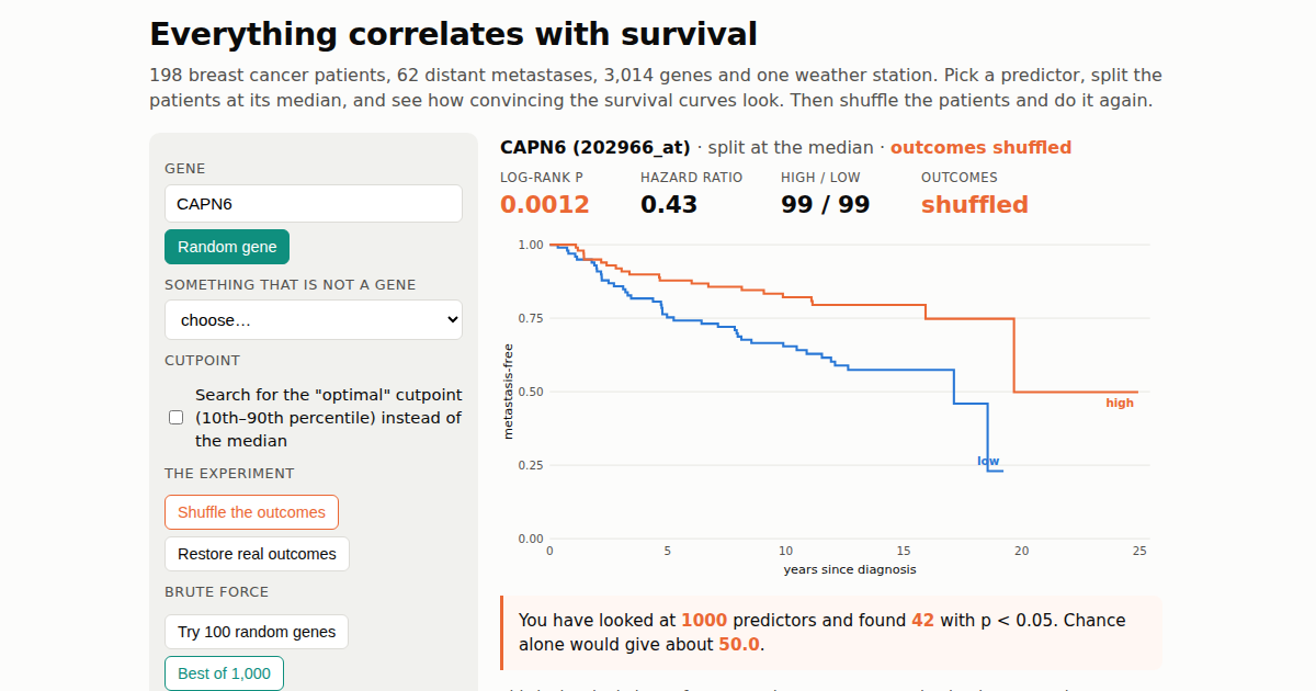
The best gene I could find in this cohort has p = 0.001. After I shuffled the patients so that no gene could possibly matter, the best gene had p = 0.0003.

I built a small thing and I would like you to play with it: Everything correlates with survival. It takes about a minute.

What it is

The data are real: 198 lymph-node-negative breast cancers from the TRANSBIG cohort (GSE7390, Desmedt et al. 2007), profiled on an Affymetrix array, with distant-metastasis-free survival as the endpoint. 62 of the 198 patients had a distant metastasis. You pick a predictor, the page splits the patients at its median, draws the two Kaplan-Meier curves, and gives you the log-rank p-value and a hazard ratio. That is the analysis behind a great many “high expression of GENE is associated with poor prognosis” figures.

You can pick from about 3,000 genes by name. You can pick ER status or tumour grade, which are real. Or you can pick the daily maximum temperature at Dublin Airport during the first half of 1990, where patient 1 is assigned 1 January, patient 2 is assigned 2 January, and so on. There are buttons to try 100 random genes at once, to pick the single best of 1,000, to swap the median split for a search over cutpoints, and, most importantly, to shuffle the outcomes so that every patient keeps their survival time but gets it reassigned at random. After a shuffle, no predictor can be related to survival. Watch what the p-values do anyway.

What you should find

At a median split with the real outcomes, 207 of the 3,014 genes on the page reach p < 0.05. That is 6.9%, against the 5% that pure chance would produce, so the arrays are carrying some real prognostic signal, spread thinly. None of the 3,014 comes close to surviving a correction for the 22,283 probes on the array (p < 0.0000022). The strongest real gene is EPHX2 at p = 0.001.

Shuffle the outcomes and 153 genes are still “significant”, three of them at p < 0.001. The strongest, MAGEA6 at p = 0.0003, beats the best real gene. If you found MAGEA6 in a genome-wide search and wrote it up, you would have a figure that looks exactly like the ones in the literature, and it would be describing a random permutation.

Tick the “optimal cutpoint” box and it gets worse in a way that deserves its own sentence. With the median split, 16 of 300 random genes reached p < 0.05 on shuffled outcomes, which is chance behaving itself. Searching each gene for the cutpoint between the 10th and 90th percentile that gives the smallest p, 122 of the same 300 did. Choosing the cutpoint by looking at the outcome turns a 5% false-positive rate into a 40% one, before any gene search on top. That is the arithmetic behind the dichotomization post, and it is why “optimal cutpoint” belongs in quotation marks.

Dublin’s weather, for the record, gives p = 0.70 at the median. It is not a prognostic factor. It could have been, one time in twenty.

What the toy is not saying

It is not saying that genes do not matter for breast cancer prognosis, or that this cohort has nothing in it. ER status splits the curves at p = 0.008, and a penalised model on all the genes together has real, modest, honestly validated predictive value, which is what the worked example later in this series is about. What it is saying is that a p-value from one split of one gene, chosen from thousands, means nothing until you know how many were looked at and how the split was chosen. The page keeps count of how many predictors you have tried, and of how many false positives that number entitles you to. Real analyses do not display that counter, and readers are left to imagine it is zero.

The page also shows something the shuffle makes vivid: a Kaplan-Meier plot with two cleanly separated arms is not evidence of anything by itself. The plot for the best shuffled gene is as pretty as any in a journal. Pretty is what a search over 1,000 candidates produces.

How it works

Everything runs in your browser. The expression values are stored as within-gene ranks, which is all a median split or a cutpoint search needs, and the whole dataset is under a megabyte. The log-rank test is implemented in about thirty lines of JavaScript, and I checked it against SciPy’s implementation on eight predictors before publishing; the chi-square statistics agree to six decimals. The build script takes the GEO series matrix and produces the data file, so the page can be regenerated for any dataset with survival times.

If you teach, the page is yours to use. Start a class on “have a go at finding a prognostic gene”, let them find one, then have them press Shuffle.

The classification versus prediction series makes the longer argument. This page is the short version.