Chapter 7 Differential Expression: DESeq2
last updated: 2023-10-27
Package Install
As usual, make sure we have the right packages for this exercise
if (!require("pacman")) install.packages("pacman"); library(pacman)

# let's load all of the files we were using and want to have again today
p_load("tidyverse", "knitr", "readr",
       "pander", "BiocManager",
       "dplyr", "stringr",
       "purrr", # for working with lists (beautify column names)
       "reactable") # for pretty tables.

# We also need these Bioconductor packages today.
p_load("DESeq2", "AnnotationDbi", "org.Sc.sgd.db")
7.1 Description
This will be our second differential expression analysis workflow, converting gene counts across samples into meaningful information about genes that appear to be significantly differentially expressed between samples. This is inspired heavily by: http://bioconductor.org/packages/devel/bioc/vignettes/DESeq2/inst/doc/DESeq2.html.
7.2 Learning outcomes
At the end of this exercise, you should be able to:
- Utilize the DESeq2 package to identify differentially expressed genes.
7.3 Loading in the featureCounts object
We saved this file at the end the exercise (Read_Counting.Rmd). Now we can load that object back in and assign it to the variable fc. Be sure to change the file path if you have saved it in a different location. This is the same way we started the edgeR analysis.
path_fc_object <- path.expand("~/Desktop/Genomic_Data_Analysis/Data/Counts/Rsubread/rsubread.yeast_fc_output.Rds")

fc <- readRDS(file = path_fc_object)
If you don’t have that file for any reason, the below code chunk will load a copy of it from Github.
counts <- read.delim('https://github.com/clstacy/GenomicDataAnalysis_Fa23/raw/main/data/ethanol_stress/counts/salmon.gene_counts.merged.nonsubsamp.tsv',
    sep = "\t",
    header = T,
    row.names = 1
  )

# clean the column names to remove the fastq.gz_quant
colnames(counts) <- str_split_fixed(counts %>% colnames(), "\\.", n = 2)[, 1]
We will create the data frame again that has all of the metadata information.
sample_metadata <- tribble(
  ~Sample,                      ~Genotype,    ~Condition,
  "YPS606_MSN24_ETOH_REP1_R1",   "msn24dd",   "EtOH",
  "YPS606_MSN24_ETOH_REP2_R1",   "msn24dd",   "EtOH",
  "YPS606_MSN24_ETOH_REP3_R1",   "msn24dd",   "EtOH",
  "YPS606_MSN24_ETOH_REP4_R1",   "msn24dd",   "EtOH",
  "YPS606_MSN24_MOCK_REP1_R1",   "msn24dd",   "unstressed",
  "YPS606_MSN24_MOCK_REP2_R1",   "msn24dd",   "unstressed",
  "YPS606_MSN24_MOCK_REP3_R1",   "msn24dd",   "unstressed",
  "YPS606_MSN24_MOCK_REP4_R1",   "msn24dd",   "unstressed",
  "YPS606_WT_ETOH_REP1_R1",      "WT",        "EtOH",
  "YPS606_WT_ETOH_REP2_R1",      "WT",        "EtOH",
  "YPS606_WT_ETOH_REP3_R1",      "WT",        "EtOH",
  "YPS606_WT_ETOH_REP4_R1",      "WT",        "EtOH",
  "YPS606_WT_MOCK_REP1_R1",      "WT",        "unstressed",
  "YPS606_WT_MOCK_REP2_R1",      "WT",        "unstressed",
  "YPS606_WT_MOCK_REP3_R1",      "WT",        "unstressed",
  "YPS606_WT_MOCK_REP4_R1",      "WT",        "unstressed") %>%
  # make Condition and Genotype a factor (with baseline as first level) for DESeq2
  mutate(
    Genotype = factor(Genotype,
                      levels = c("WT", "msn24dd")),
    Condition = factor(Condition,
                       levels = c("unstressed", "EtOH"))
  )
7.4 Count loading and Annotation
The count matrix is used to construct a DESeqDataSet class object. This is the main data class in the DESeq2 package. The DESeqDataSet object is used to store all the information required to fit a generalized linear model to the data, including library sizes and dispersion estimates as well as counts for each gene.
Because we used the featureCounts function (Liao, Smyth, and Shi 2013) in the Rsubread package, the matrix of read counts can be directly provided from the "counts" element in the list output. The count matrix and column data can typically be read into R from flat files using base R functions such as read.csv or read.delim.
With the count matrix, cts, and the sample information, coldata, we can construct a DESeqDataSet:
# notice the different design specification
dds <- DESeqDataSetFromMatrix(countData = round(counts),
                              colData = sample_metadata,
                              design = ~ 1 + Genotype + Condition + Genotype:Condition)
## converting counts to integer mode# simplify the column names to make them pretty
colnames(dds) <- str_split_fixed(colnames(dds), "\\.", n = 2)[, 1]
# take a look at the dds object
dds## class: DESeqDataSet
## dim: 6571 16
## metadata(1): version
## assays(1): counts
## rownames(6571): YIL170W YIL175W ... YJL134W YER096W
## rowData names(0):
## colnames(16): YPS606_MSN24_ETOH_REP1_R1 YPS606_MSN24_ETOH_REP2_R1 ...
## YPS606_WT_MOCK_REP3_R1 YPS606_WT_MOCK_REP4_R1
## colData names(3): Sample Genotype Condition7.5 Filtering to remove low counts
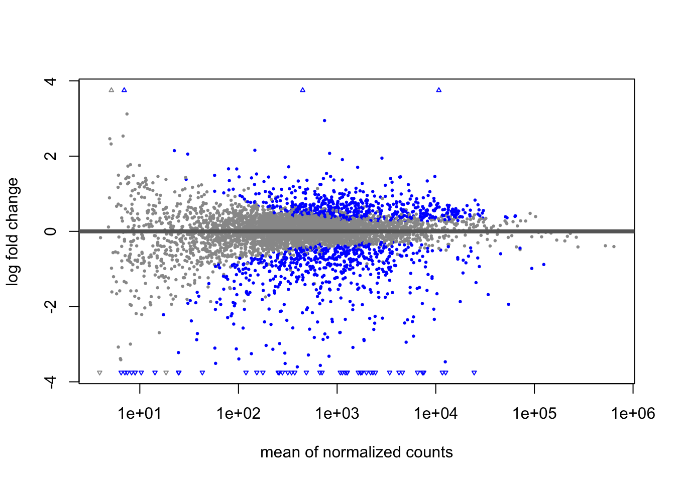
While it is not necessary to pre-filter low count genes before running the DESeq2 functions, there are two reasons which make pre-filtering useful: by removing rows in which there are very few reads, we reduce the memory size of the dds data object, and we increase the speed of count modeling within DESeq2. It can also improve visualizations, as features with no information for differential expression are not plotted in dispersion plots or MA-plots.
Here we perform pre-filtering to keep only rows that have a count of at least 10 for a minimal number of samples. The count of 10 is a reasonable choice for bulk RNA-seq. A recommendation for the minimal number of samples is to specify the smallest group size, e.g. here there are 4 treated samples. If there are not discrete groups, one can use the minimal number of samples where non-zero counts would be considered interesting. One can also omit this step entirely and just rely on the independent filtering procedures available in results(), either IHW or genefilter. See independent filtering section.
7.6 Testing for differential expression
The standard differential expression analysis steps are wrapped into a single function, DESeq. The estimation steps performed by this function are described below, in the manual page for ?DESeq and in the Methods section of the DESeq2 publication (Love, Huber, and Anders 2014).
Results tables are generated using the function results, which extracts a results table with log2 fold changes, p values and adjusted p values. With no additional arguments to results, the log2 fold change and Wald test p value will be for the last variable in the design formula, and if this is a factor, the comparison will be the last level of this variable over the reference level However, the order of the variables of the design do not matter so long as the user specifies the comparison to build a results table for, using the name or contrast arguments of results.
Details about the comparison are printed to the console, directly above the results table. The text, condition treated vs untreated, tells you that the estimates are of the logarithmic fold change log2(treated/untreated).
## estimating size factors## estimating dispersions## gene-wise dispersion estimates## mean-dispersion relationship## final dispersion estimates## fitting model and testing## [1] "Intercept" "Genotype_msn24dd_vs_WT"
## [3] "Condition_EtOH_vs_unstressed" "Genotypemsn24dd.ConditionEtOH"# create a model matrix
mod_mat <- model.matrix(design(dds), colData(dds))
# define coefficient vectors for each group
WT_MOCK <- colMeans(mod_mat[dds$Genotype == "WT" & dds$Condition == "unstressed", ])
WT_EtOH <- colMeans(mod_mat[dds$Genotype == "WT" & dds$Condition == "EtOH", ])
MSN24_MOCK <- colMeans(mod_mat[dds$Genotype == "msn24dd" & dds$Condition == "unstressed", ])
MSN24dd_EtOH <- colMeans(mod_mat[dds$Genotype == "msn24dd" & dds$Condition == "EtOH", ])The nice thing about this approach is that we do not need to worry about any of this, the weights come from our colMeans() call automatically. And now, any contrasts that we make will take these weights into account:
## log2 fold change (MLE): Genotypemsn24dd.ConditionEtOH
## Wald test p-value: Genotypemsn24dd.ConditionEtOH
## DataFrame with 5622 rows and 6 columns
##            baseMean log2FoldChange     lfcSE      stat      pvalue        padj
##           <numeric>      <numeric> <numeric> <numeric>   <numeric>   <numeric>
## YIL170W     14.8499      0.9768970  0.878689  1.111767 2.66238e-01 0.443362781
## YFL056C    265.8871      0.8156191  0.183405  4.447097 8.70386e-06 0.000074707
## YAR061W     20.1326     -0.6364363  0.468363 -1.358852 1.74194e-01 0.329294856
## YGR014W   2615.6548     -0.0174106  0.128224 -0.135782 8.91994e-01 0.942098024
## YPR031W    237.3713     -0.1163443  0.226110 -0.514547 6.06870e-01 0.755325201
## ...             ...            ...       ...       ...         ...         ...
## YDL086C-A   15.0128     -0.7051445  0.626958  -1.12471  0.26071321  0.43661890
## YJR067C    145.6068     -0.0844778  0.213231  -0.39618  0.69197231  0.81490383
## YDR030C     80.1245     -0.3096978  0.281000  -1.10213  0.27040547  0.44831011
## YJL134W   1389.3306      0.2569824  0.147556   1.74159  0.08157979  0.19181998
## YER096W    250.0039     -0.6634104  0.214676  -3.09029  0.00199959  0.00931377
We could have equivalently produced this results table with the following more specific command. Because Genotypemsn24dd:ConditionEtOH is the last variable in the design, we could optionally leave off the contrast argument to extract the comparison of the two levels of Genotypemsn24dd:ConditionEtOH.
res %>%
  data.frame() %>%
  rownames_to_column("ORF") %>%
  # add the gene names
  left_join(AnnotationDbi::select(org.Sc.sgd.db,keys=.$ORF,columns="GENENAME"),by="ORF") %>%
  relocate(GENENAME, .after = ORF) %>%
  arrange(padj) %>%
  mutate(log2FoldChange = round(log2FoldChange, 2)) %>%
  mutate(across(where(is.numeric), signif, 3)) %>%
  reactable(
    searchable = TRUE,
    showSortable = TRUE,
    columns = list(ORF = colDef(
      cell = function(value) {
        # Render as a link
        url <-
          sprintf("https://www.yeastgenome.org/locus/%s", value)
        htmltools::tags$a(href = url, target = "_blank", as.character(value))
      }
    ))
  )
## 'select()' returned 1:1 mapping between keys and columns## Warning: There was 1 warning in `mutate()`.
## ℹ In argument: `across(where(is.numeric), signif, 3)`.
## Caused by warning:
## ! The `...` argument of `across()` is deprecated as of dplyr 1.1.0.
## Supply arguments directly to `.fns` through an anonymous function instead.
##
## # Previously
## across(a:b, mean, na.rm = TRUE)
##
## # Now
## across(a:b, \(x) mean(x, na.rm = TRUE))# filter based on padj and a lfc cutoff
res_sig <- subset(res, padj<.01)
res_lfc <- subset(res_sig, abs(log2FoldChange) > 1)##
## out of 5622 with nonzero total read count
## adjusted p-value < 0.05
## LFC > 0 (up) : 832, 15%
## LFC < 0 (down) : 815, 14%
## outliers [1] : 0, 0%
## low counts [2] : 0, 0%
## (mean count < 4)
## [1] see 'cooksCutoff' argument of ?results
## [2] see 'independentFiltering' argument of ?results##
## out of 354 with nonzero total read count
## adjusted p-value < 0.05
## LFC > 0 (up) : 76, 21%
## LFC < 0 (down) : 278, 79%
## outliers [1] : 0, 0%
## low counts [2] : 0, 0%
## (mean count < 4)
## [1] see 'cooksCutoff' argument of ?results
## [2] see 'independentFiltering' argument of ?results## log2 fold change (MLE): 0,0,0,+1
## Wald test p-value: 0,0,0,+1
## DataFrame with 6 rows and 6 columns
## baseMean log2FoldChange lfcSE stat pvalue padj
## <numeric> <numeric> <numeric> <numeric> <numeric> <numeric>
## YER091C 2846.4044 1.94771 0.267390 7.28414 3.23735e-13 8.42610e-12
## YJR127C 819.0282 -1.34748 0.150234 -8.96917 2.98759e-19 1.21712e-17
## YAL040C 3530.0007 -1.05979 0.141324 -7.49903 6.42942e-14 1.78941e-12
## YLR456W 57.3756 1.06661 0.333378 3.19940 1.37712e-03 6.76761e-03
## YMR173W 295.1969 -3.23614 0.268425 -12.05605 1.80230e-33 1.49008e-31
## YFR017C 252.8558 -5.39554 0.489053 -11.03265 2.65916e-28 1.84565e-26Let’s take a quick look at the differential expression
 Plot an individual gene:
gene <- "YER091C"

# Here is the default visualization. Depending on screen size, the xlab
# might not show all of the groups.
plotCounts(dds, gene="YEL039C", intgroup=c("Genotype","Condition"),
           xlab="Genotype:Condition")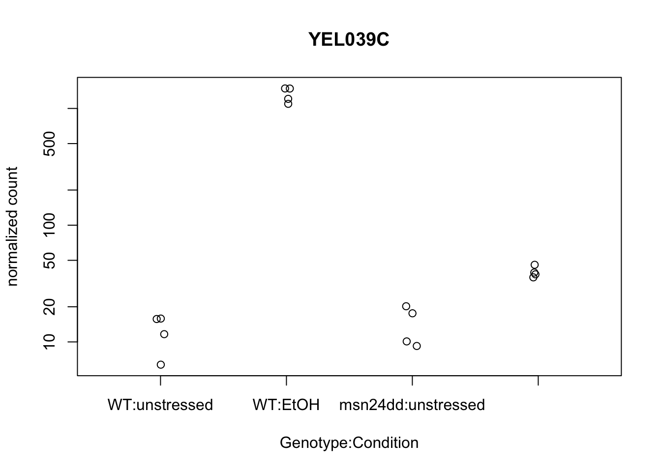
# Make the plot prettier with ggplot(). Note the returnData=TRUE let's us do this.
plotCounts(dds, gene=gene, intgroup=c("Genotype","Condition"),
           xlab="Genotype:Condition", returnData = TRUE) %>%
  rownames_to_column("Sample") %>%
  ggplot(aes(x=Genotype, y=count, color=Condition, shape=Condition)) +
  geom_dotplot(binaxis = "y", stackdir = "center", dotsize=0.75,
               position=position_dodge(0.4), # this seperates by Condition a bit
               fill=NA) +
  labs(x="Genotype",
       y="normalized count",
       title=paste0("Visualizing the expression of ORF: ", gene)
       ) +
  scale_y_log10() +
  theme_classic()
## Bin width defaults to 1/30 of the range of the data. Pick better value with
## `binwidth`.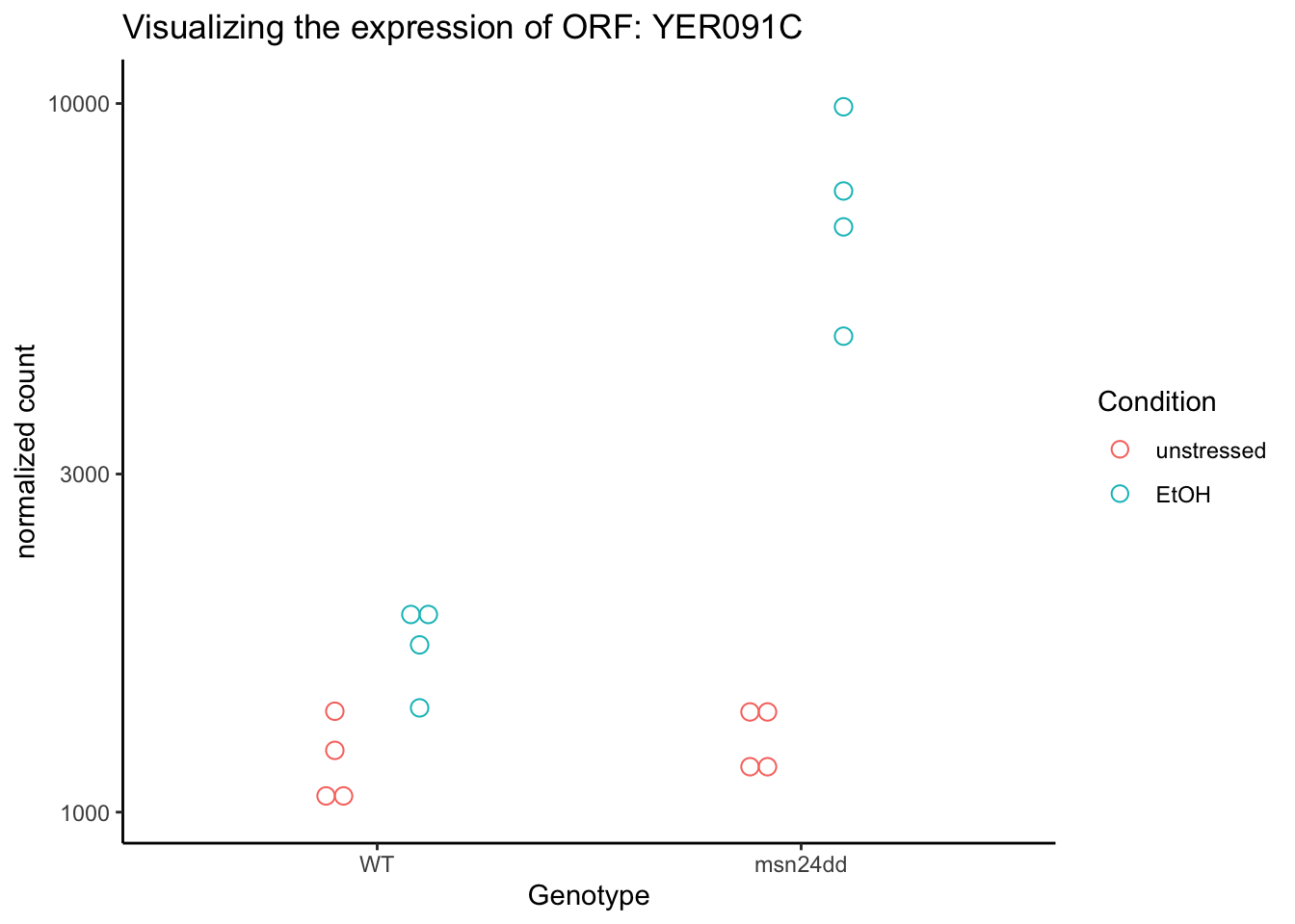
We need to make sure and save our output file(s).
# Choose topTags destination
dir_output_DESeq2 <-
  path.expand("~/Desktop/Genomic_Data_Analysis/Analysis/DESeq2/")
if (!dir.exists(dir_output_DESeq2)) {
  dir.create(dir_output_DESeq2, recursive = TRUE)
}

# for sharing with others, a tsv for the res output is convenient.
# Depending on what people need, we can save res object as is or beautify it.
res %>%
  data.frame() %>%
  rownames_to_column("ORF") %>%
  left_join(AnnotationDbi::select(org.Sc.sgd.db,keys=.$ORF,columns="GENENAME"),by="ORF") %>%
  relocate(GENENAME, .after = ORF) %>%
  # arrange(padj) %>%
  # mutate(log2FoldChange = round(log2FoldChange, 2)) %>%
  # mutate(across(where(is.numeric), signif, 3)) %>%
  write_tsv(., file = paste0(dir_output_DESeq2, "yeast_res_DESeq2.tsv"))
## 'select()' returned 1:1 mapping between keys and columns7.7 Questions
Question 1: How many genes were upregulated and downregulated in the contrast we looked at in this activity? Be sure to clarify the cutoffs used for determining significance.
Question 2: Choose one of the contrasts in my.contrasts that we didn’t test together, and identify the top 3 most differentially expressed genes.
Question 3: In the contrast you chose, give a brief description of the biological interpretation of that contrast.
Question 4: We analyzed differential expression of the counts generated by the full Salmon counts. Load in the counts generated by using the subset samples and look at the same contrast we did in class. What differences and similarities do you see?
A template for doing this is below:
path_subset_counts <- path.expand("~/Desktop/Genomic_Data_Analysis/Data/Counts/Salmon/salmon.gene_counts.merged.yeast.tsv")

# If you don't have thot file, uncomment the code below and run it instead.
# read.delim('https://github.com/clstacy/GenomicDataAnalysis_Fa23/raw/main/data/ethanol_stress/counts/salmon.gene_counts.merged.yeast.tsv', sep = "\t", header = T, row.names = 1)


subset_counts <- read.delim(file = path_subset_counts,
    sep = "\t",
    header = T,
    row.names = 1
  )
# We are reusing the sample_metadata, group, etc that we assigned above
# create DESeqDataSet with salmon counts (round needed for nonintegers)
dds_subset <- DESeqDataSetFromMatrix(countData = round(subset_counts),
colData = sample_metadata,
design = ~ 1 + Genotype + Condition + Genotype:Condition)## converting counts to integer mode# simplify the column names to make them pretty
colnames(dds_subset) <- str_split_fixed(colnames(dds_subset), "\\.", n = 2)[, 1]
# filter low counts
keep_subset <- rowSums(counts(dds_subset) >= 10) >= smallestGroupSize
dds_subset <- dds_subset[keep_subset,]
# generate the fit
dds_subset <- DESeq(dds_subset)## estimating size factors## estimating dispersions## gene-wise dispersion estimates## mean-dispersion relationship## final dispersion estimates## fitting model and testing# test our contrast of interest
res_subset <- results(dds_subset,
contrast = (MSN24dd_EtOH - MSN24_MOCK) - (WT_EtOH - WT_MOCK)
)
# generate a beautiful table for the pdf/html file.
res_subset %>%
data.frame() %>%
rownames_to_column("ORF") %>%
# add the gene names
left_join(AnnotationDbi::select(org.Sc.sgd.db,keys=.$ORF,columns="GENENAME"),by="ORF") %>%
relocate(GENENAME, .after = ORF) %>%
arrange(padj) %>%
mutate(log2FoldChange = round(log2FoldChange, 2)) %>%
mutate(across(where(is.numeric), signif, 3)) %>%
reactable(
searchable = TRUE,
showSortable = TRUE,
columns = list(ORF = colDef(
cell = function(value) {
# Render as a link
url <-
sprintf("https://www.yeastgenome.org/locus/%s", value)
htmltools::tags$a(href = url, target = "_blank", as.character(value))
}
))
)## 'select()' returned 1:1 mapping between keys and columns##
## out of 2542 with nonzero total read count
## adjusted p-value < 0.05
## LFC > 0 (up) : 76, 3%
## LFC < 0 (down) : 99, 3.9%
## outliers [1] : 0, 0%
## low counts [2] : 690, 27%
## (mean count < 10)
## [1] see 'cooksCutoff' argument of ?results
## [2] see 'independentFiltering' argument of ?results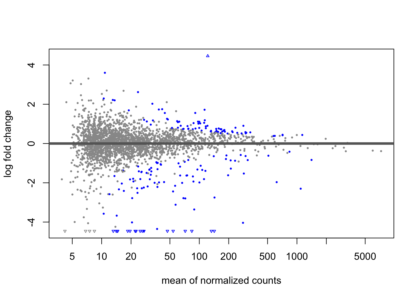 Be sure to knit this file into a pdf or html file once you’re finished.
System information for reproducibility:
R version 4.3.1 (2023-06-16)
Platform: aarch64-apple-darwin20 (64-bit)
locale: en_US.UTF-8||en_US.UTF-8||en_US.UTF-8||C||en_US.UTF-8||en_US.UTF-8
attached base packages: stats4, stats, graphics, grDevices, utils, datasets, methods and base
other attached packages: DESeq2(v.1.40.2), edgeR(v.3.42.4), limma(v.3.56.2), reactable(v.0.4.4), webshot2(v.0.1.1), statmod(v.1.5.0), Rsubread(v.2.14.2), ShortRead(v.1.58.0), GenomicAlignments(v.1.36.0), SummarizedExperiment(v.1.30.2), MatrixGenerics(v.1.12.3), matrixStats(v.1.0.0), Rsamtools(v.2.16.0), GenomicRanges(v.1.52.1), Biostrings(v.2.68.1), GenomeInfoDb(v.1.36.4), XVector(v.0.40.0), BiocParallel(v.1.34.2), Rfastp(v.1.10.0), org.Sc.sgd.db(v.3.17.0), AnnotationDbi(v.1.62.2), IRanges(v.2.34.1), S4Vectors(v.0.38.2), Biobase(v.2.60.0), BiocGenerics(v.0.46.0), clusterProfiler(v.4.8.2), ggVennDiagram(v.1.2.3), tidytree(v.0.4.5), igraph(v.1.5.1), janitor(v.2.2.0), BiocManager(v.1.30.22), pander(v.0.6.5), knitr(v.1.44), here(v.1.0.1), lubridate(v.1.9.3), forcats(v.1.0.0), stringr(v.1.5.0), dplyr(v.1.1.3), purrr(v.1.0.2), readr(v.2.1.4), tidyr(v.1.3.0), tibble(v.3.2.1), ggplot2(v.3.4.4), tidyverse(v.2.0.0) and pacman(v.0.5.1)
loaded via a namespace (and not attached): splines(v.4.3.1), later(v.1.3.1), bitops(v.1.0-7), ggplotify(v.0.1.2), polyclip(v.1.10-6), lifecycle(v.1.0.3), rprojroot(v.2.0.3), vroom(v.1.6.4), processx(v.3.8.2), lattice(v.0.21-9), MASS(v.7.3-60), crosstalk(v.1.2.0), magrittr(v.2.0.3), sass(v.0.4.7), rmarkdown(v.2.25), jquerylib(v.0.1.4), yaml(v.2.3.7), cowplot(v.1.1.1), chromote(v.0.1.2), DBI(v.1.1.3), RColorBrewer(v.1.1-3), abind(v.1.4-5), zlibbioc(v.1.46.0), ggraph(v.2.1.0), RCurl(v.1.98-1.12), yulab.utils(v.0.1.0), tweenr(v.2.0.2), GenomeInfoDbData(v.1.2.10), enrichplot(v.1.20.0), ggrepel(v.0.9.4), codetools(v.0.2-19), DelayedArray(v.0.26.7), DOSE(v.3.26.1), ggforce(v.0.4.1), tidyselect(v.1.2.0), aplot(v.0.2.2), farver(v.2.1.1), viridis(v.0.6.4), jsonlite(v.1.8.7), ellipsis(v.0.3.2), tidygraph(v.1.2.3), tools(v.4.3.1), treeio(v.1.24.3), Rcpp(v.1.0.11), glue(v.1.6.2), gridExtra(v.2.3), xfun(v.0.40), qvalue(v.2.32.0), websocket(v.1.4.1), withr(v.2.5.1), fastmap(v.1.1.1), latticeExtra(v.0.6-30), fansi(v.1.0.5), digest(v.0.6.33), timechange(v.0.2.0), R6(v.2.5.1), gridGraphics(v.0.5-1), colorspace(v.2.1-0), GO.db(v.3.17.0), jpeg(v.0.1-10), RSQLite(v.2.3.1), utf8(v.1.2.3), generics(v.0.1.3), data.table(v.1.14.8), graphlayouts(v.1.0.1), httr(v.1.4.7), htmlwidgets(v.1.6.2), S4Arrays(v.1.0.6), scatterpie(v.0.2.1), pkgconfig(v.2.0.3), gtable(v.0.3.4), blob(v.1.2.4), hwriter(v.1.3.2.1), shadowtext(v.0.1.2), htmltools(v.0.5.6.1), bookdown(v.0.36), fgsea(v.1.26.0), scales(v.1.2.1), png(v.0.1-8), snakecase(v.0.11.1), ggfun(v.0.1.3), rstudioapi(v.0.15.0), tzdb(v.0.4.0), reshape2(v.1.4.4), rjson(v.0.2.21), nlme(v.3.1-163), cachem(v.1.0.8), RVenn(v.1.1.0), parallel(v.4.3.1), HDO.db(v.0.99.1), pillar(v.1.9.0), grid(v.4.3.1), vctrs(v.0.6.4), promises(v.1.2.1), archive(v.1.1.5), evaluate(v.0.22), cli(v.3.6.1), locfit(v.1.5-9.8), compiler(v.4.3.1), rlang(v.1.1.1), crayon(v.1.5.2), reactR(v.0.5.0), interp(v.1.1-4), ps(v.1.7.5), plyr(v.1.8.9), fs(v.1.6.3), stringi(v.1.7.12), viridisLite(v.0.4.2), deldir(v.1.0-9), munsell(v.0.5.0), lazyeval(v.0.2.2), GOSemSim(v.2.26.1), Matrix(v.1.6-1.1), hms(v.1.1.3), patchwork(v.1.1.3), bit64(v.4.0.5), KEGGREST(v.1.40.1), memoise(v.2.0.1), bslib(v.0.5.1), ggtree(v.3.8.2), fastmatch(v.1.1-4), bit(v.4.0.5), downloader(v.0.4), ape(v.5.7-1) and gson(v.0.1.0)