Chapter 8 Differential Expression: limma
last updated: 2023-10-27
Install Packages
As usual, make sure we have the right packages for this exercise
if (!require("pacman")) install.packages("pacman"); library(pacman)

# let's load all of the files we were using and want to have again today
p_load("tidyverse", "knitr", "readr",
       "pander", "BiocManager",
       "dplyr", "stringr",
       "statmod", # required dependency, need to load manually on some macOS versions.
       "Glimma", # beautifies limma results
       "purrr", # for working with lists (beautify column names)
       "reactable") # for pretty tables.

# We also need these Bioconductor packages today.
p_load("edgeR", "AnnotationDbi", "org.Sc.sgd.db", "ggVennDiagram")
#NOTE: edgeR loads limma as a dependency
8.1 Description
This will be our last differential expression analysis workflow, converting gene counts across samples into meaningful information about genes that appear to be significantly differentially expressed between samples
8.2 Learning Objectives
At the end of this exercise, you should be able to:
- Generate a table of sample metadata.
- Filter low counts and normalize count data.
- Utilize the limma package to identify differentially expressed genes.
8.3 Loading in the count data file
We are downloading the counts for the non-subsampled fastq files from a
Github repository using the code below. Just as in previous exercises,
assign the data to the variable counts. You can change the file path
if you have saved it to your computer in a different location.
counts <- read.delim('https://github.com/clstacy/GenomicDataAnalysis_Fa23/raw/main/data/ethanol_stress/counts/salmon.gene_counts.merged.nonsubsamp.tsv',
    sep = "\t",
    header = T,
    row.names = 1
  )
If you don’t have that file for any reason, the below code chunk will load a copy of it from Github.
To find the order of files we need, we can get just the part of the column name before the first “.” symbol with this command:
##  [1] "YPS606_MSN24_ETOH_REP1_R1" "YPS606_MSN24_ETOH_REP2_R1"
##  [3] "YPS606_MSN24_ETOH_REP3_R1" "YPS606_MSN24_ETOH_REP4_R1"
##  [5] "YPS606_MSN24_MOCK_REP1_R1" "YPS606_MSN24_MOCK_REP2_R1"
##  [7] "YPS606_MSN24_MOCK_REP3_R1" "YPS606_MSN24_MOCK_REP4_R1"
##  [9] "YPS606_WT_ETOH_REP1_R1"    "YPS606_WT_ETOH_REP2_R1"
## [11] "YPS606_WT_ETOH_REP3_R1"    "YPS606_WT_ETOH_REP4_R1"
## [13] "YPS606_WT_MOCK_REP1_R1"    "YPS606_WT_MOCK_REP2_R1"
## [15] "YPS606_WT_MOCK_REP3_R1"    "YPS606_WT_MOCK_REP4_R1"
sample_metadata <- tribble(
~Sample, ~Genotype, ~Condition,
"YPS606_MSN24_ETOH_REP1_R1", "msn24dd", "EtOH",
"YPS606_MSN24_ETOH_REP2_R1", "msn24dd", "EtOH",
"YPS606_MSN24_ETOH_REP3_R1", "msn24dd", "EtOH",
"YPS606_MSN24_ETOH_REP4_R1", "msn24dd", "EtOH",
"YPS606_MSN24_MOCK_REP1_R1", "msn24dd", "unstressed",
"YPS606_MSN24_MOCK_REP2_R1", "msn24dd", "unstressed",
"YPS606_MSN24_MOCK_REP3_R1", "msn24dd", "unstressed",
"YPS606_MSN24_MOCK_REP4_R1", "msn24dd", "unstressed",
"YPS606_WT_ETOH_REP1_R1", "WT", "EtOH",
"YPS606_WT_ETOH_REP2_R1", "WT", "EtOH",
"YPS606_WT_ETOH_REP3_R1", "WT", "EtOH",
"YPS606_WT_ETOH_REP4_R1", "WT", "EtOH",
"YPS606_WT_MOCK_REP1_R1", "WT", "unstressed",
"YPS606_WT_MOCK_REP2_R1", "WT", "unstressed",
"YPS606_WT_MOCK_REP3_R1", "WT", "unstressed",
"YPS606_WT_MOCK_REP4_R1", "WT", "unstressed") %>%
# Create a new column that combines the Genotype and Condition value
mutate(Group = factor(
paste(Genotype, Condition, sep = "."),
levels = c(
"WT.unstressed","WT.EtOH",
"msn24dd.unstressed", "msn24dd.EtOH"
)
)) %>%
# make Condition and Genotype a factor (with baseline as first level) for edgeR
mutate(
Genotype = factor(Genotype,
levels = c("WT", "msn24dd")),
Condition = factor(Condition,
levels = c("unstressed", "EtOH"))
)Now, let’s create a design matrix with this information
group <- sample_metadata$Group
design <- model.matrix(~ 0 + group)

# beautify column names
colnames(design) <- levels(group)
design
## WT.unstressed WT.EtOH msn24dd.unstressed msn24dd.EtOH
## 1 0 0 0 1
## 2 0 0 0 1
## 3 0 0 0 1
## 4 0 0 0 1
## 5 0 0 1 0
## 6 0 0 1 0
## 7 0 0 1 0
## 8 0 0 1 0
## 9 0 1 0 0
## 10 0 1 0 0
## 11 0 1 0 0
## 12 0 1 0 0
## 13 1 0 0 0
## 14 1 0 0 0
## 15 1 0 0 0
## 16 1 0 0 0
## attr(,"assign")
## [1] 1 1 1 1
## attr(,"contrasts")
## attr(,"contrasts")$group
## [1] "contr.treatment"8.4 Count loading and Annotation
The count matrix is used to construct a DGEList class object. This is the main data class in the edgeR package. The DGEList object is used to store all the information required to fit a generalized linear model to the data, including library sizes and dispersion estimates as well as counts for each gene.
##                                        group lib.size norm.factors
## YPS606_MSN24_ETOH_REP1_R1       msn24dd.EtOH 17409481            1
## YPS606_MSN24_ETOH_REP2_R1       msn24dd.EtOH 14055425            1
## YPS606_MSN24_ETOH_REP3_R1       msn24dd.EtOH 13127876            1
## YPS606_MSN24_ETOH_REP4_R1       msn24dd.EtOH 16655559            1
## YPS606_MSN24_MOCK_REP1_R1 msn24dd.unstressed 12266723            1
## YPS606_MSN24_MOCK_REP2_R1 msn24dd.unstressed 11781244            1
## YPS606_MSN24_MOCK_REP3_R1 msn24dd.unstressed 11340274            1
## YPS606_MSN24_MOCK_REP4_R1 msn24dd.unstressed 13024330            1
## YPS606_WT_ETOH_REP1_R1               WT.EtOH 15422048            1
## YPS606_WT_ETOH_REP2_R1               WT.EtOH 14924728            1
## YPS606_WT_ETOH_REP3_R1               WT.EtOH 14738753            1
## YPS606_WT_ETOH_REP4_R1               WT.EtOH 12203133            1
## YPS606_WT_MOCK_REP1_R1         WT.unstressed 13592206            1
## YPS606_WT_MOCK_REP2_R1         WT.unstressed 12921965            1
## YPS606_WT_MOCK_REP3_R1         WT.unstressed 13128396            1
## YPS606_WT_MOCK_REP4_R1         WT.unstressed 15568155            1
Human-readable gene symbols can also be added to complement the gene ID for each gene, using the annotation in the org.Sc.sgd.db package.
## 'select()' returned 1:1 mapping between keys and columns## ORF SGD GENENAME
## 1 YIL170W S000001432 HXT12
## 2 YIL175W S000001437 <NA>
## 3 YPL276W S000006197 <NA>
## 4 YFL056C S000001838 AAD6
## 5 YCL074W S000000579 <NA>
## 6 YAR061W S000000087 <NA>8.5 Filtering to remove low counts
Genes with very low counts across all libraries provide little evidence for differential ex- pression. In addition, the pronounced discreteness of these counts interferes with some of the statistical approximations that are used later in the pipeline. These genes should be filtered out prior to further analysis. Here, we will retain a gene only if it is expressed at a count-per-million (CPM) above 60 in at least four samples.
##    Mode   FALSE    TRUE
## logical     956    5615
Where did those cutoff numbers come from?
As a general rule, we don’t want to exclude a gene that is expressed in only one group, so a cutoff number equal to the number of replicates can be a good starting point. For counts, a good threshold can be chosen by identifying the CPM that corresponds to a count of 10, which in this case would be about 60 (due to our fastq files being subsets of the full reads):
##      [,1]
## [1,] 0.72
Smaller CPM thresholds are usually appropriate for larger libraries.
8.6 Normalization for composition bias
TMM normalization is performed to eliminate composition biases between libraries. This generates a set of normalization factors, where the product of these factors and the library sizes defines the effective library size. The calcNormFactors function returns the DGEList argument with only the norm.factors changed.
## group lib.size norm.factors
## YPS606_MSN24_ETOH_REP1_R1 msn24dd.EtOH 17409481 1.239
## YPS606_MSN24_ETOH_REP2_R1 msn24dd.EtOH 14055425 1.102
## YPS606_MSN24_ETOH_REP3_R1 msn24dd.EtOH 13127876 1.108
## YPS606_MSN24_ETOH_REP4_R1 msn24dd.EtOH 16655559 1.007
## YPS606_MSN24_MOCK_REP1_R1 msn24dd.unstressed 12266723 1.038
## YPS606_MSN24_MOCK_REP2_R1 msn24dd.unstressed 11781244 1.003
## YPS606_MSN24_MOCK_REP3_R1 msn24dd.unstressed 11340274 0.960
## YPS606_MSN24_MOCK_REP4_R1 msn24dd.unstressed 13024330 0.984
## YPS606_WT_ETOH_REP1_R1 WT.EtOH 15422048 0.839
## YPS606_WT_ETOH_REP2_R1 WT.EtOH 14924728 0.941
## YPS606_WT_ETOH_REP3_R1 WT.EtOH 14738753 0.988
## YPS606_WT_ETOH_REP4_R1 WT.EtOH 12203133 0.971
## YPS606_WT_MOCK_REP1_R1 WT.unstressed 13592206 0.990
## YPS606_WT_MOCK_REP2_R1 WT.unstressed 12921965 1.038
## YPS606_WT_MOCK_REP3_R1 WT.unstressed 13128396 0.900
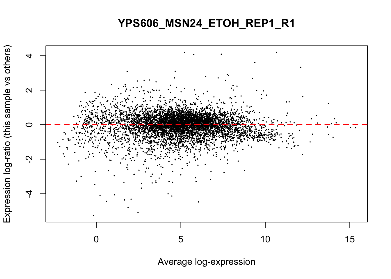
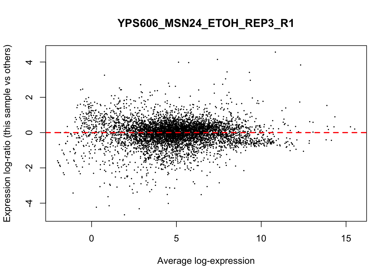
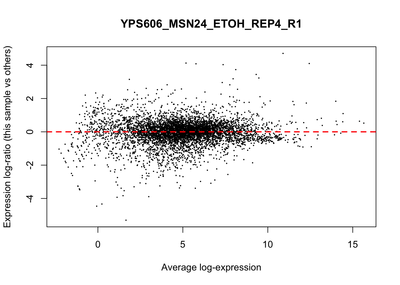
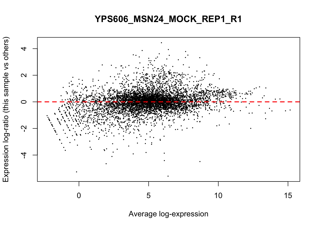
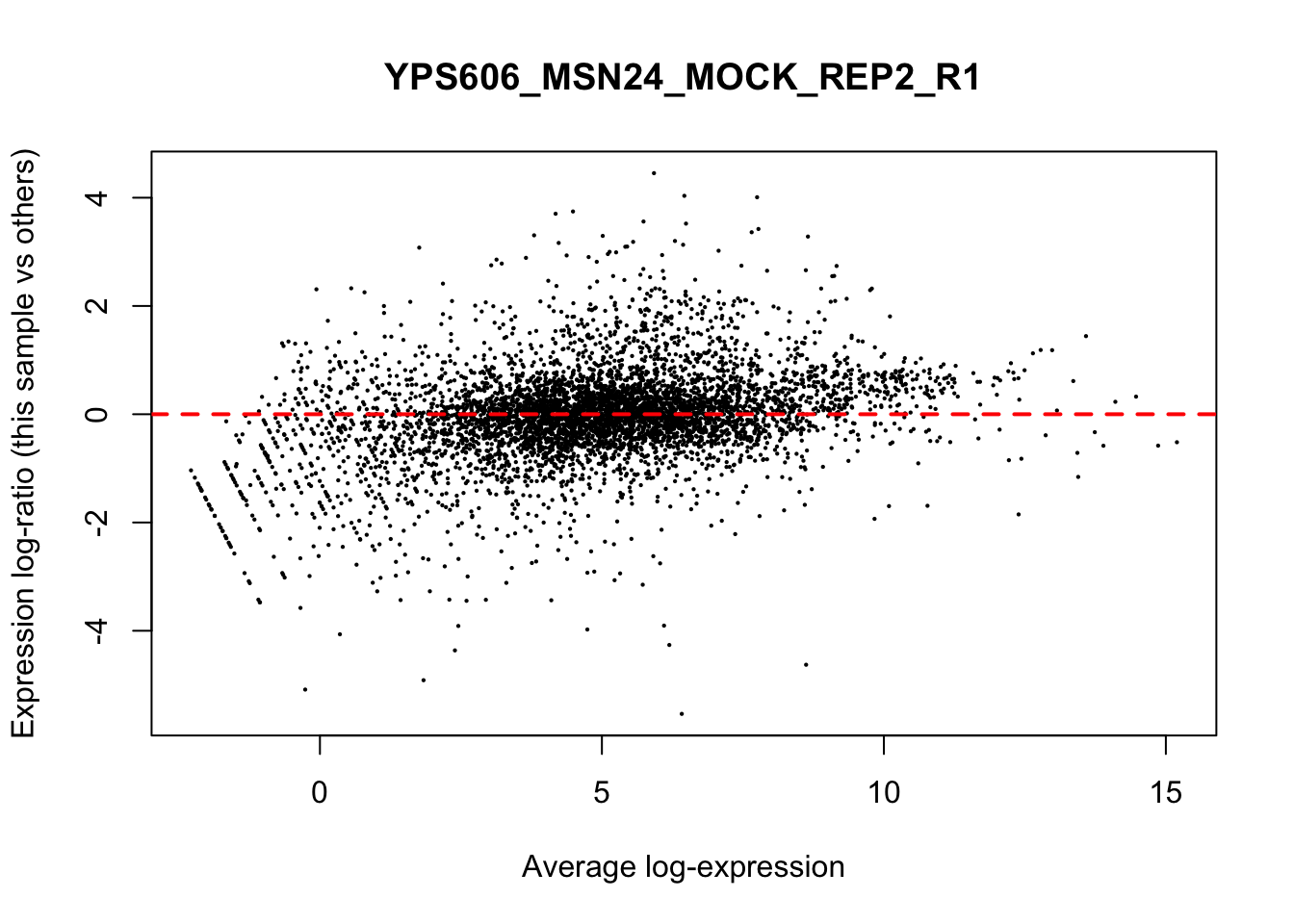
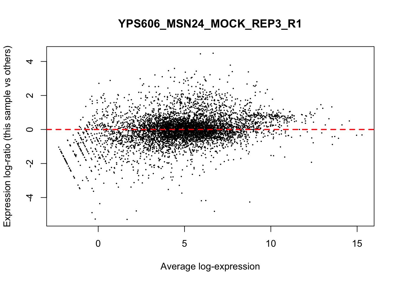
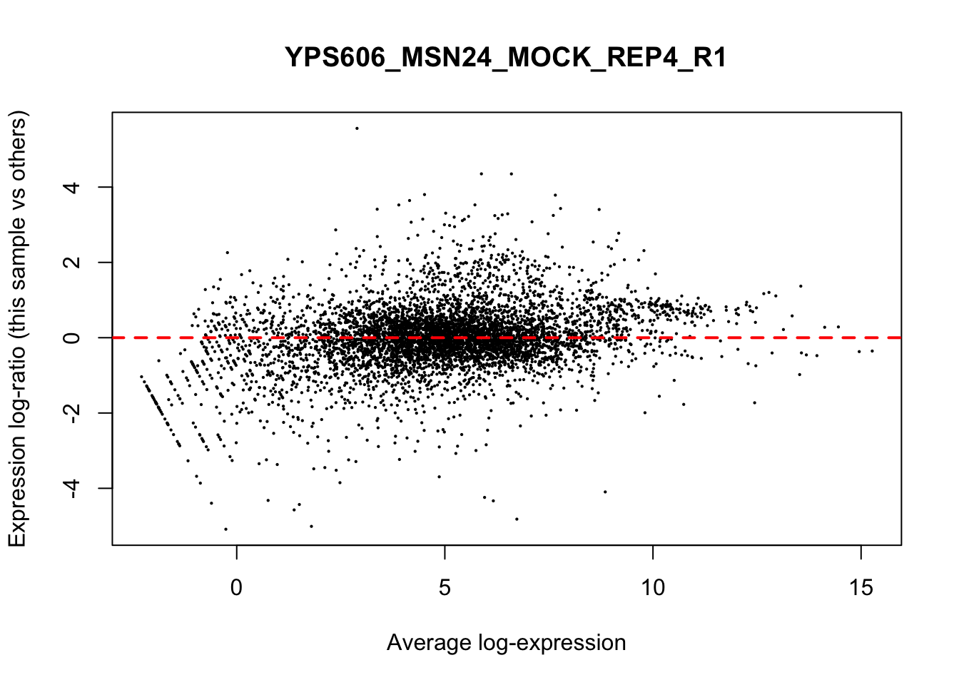
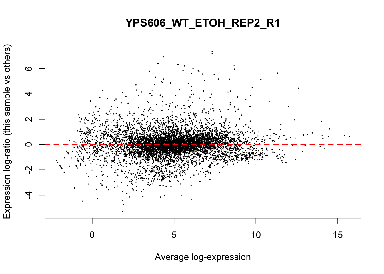
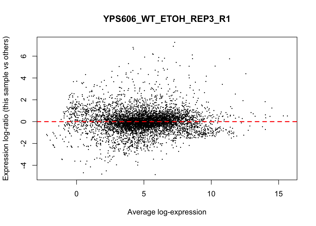
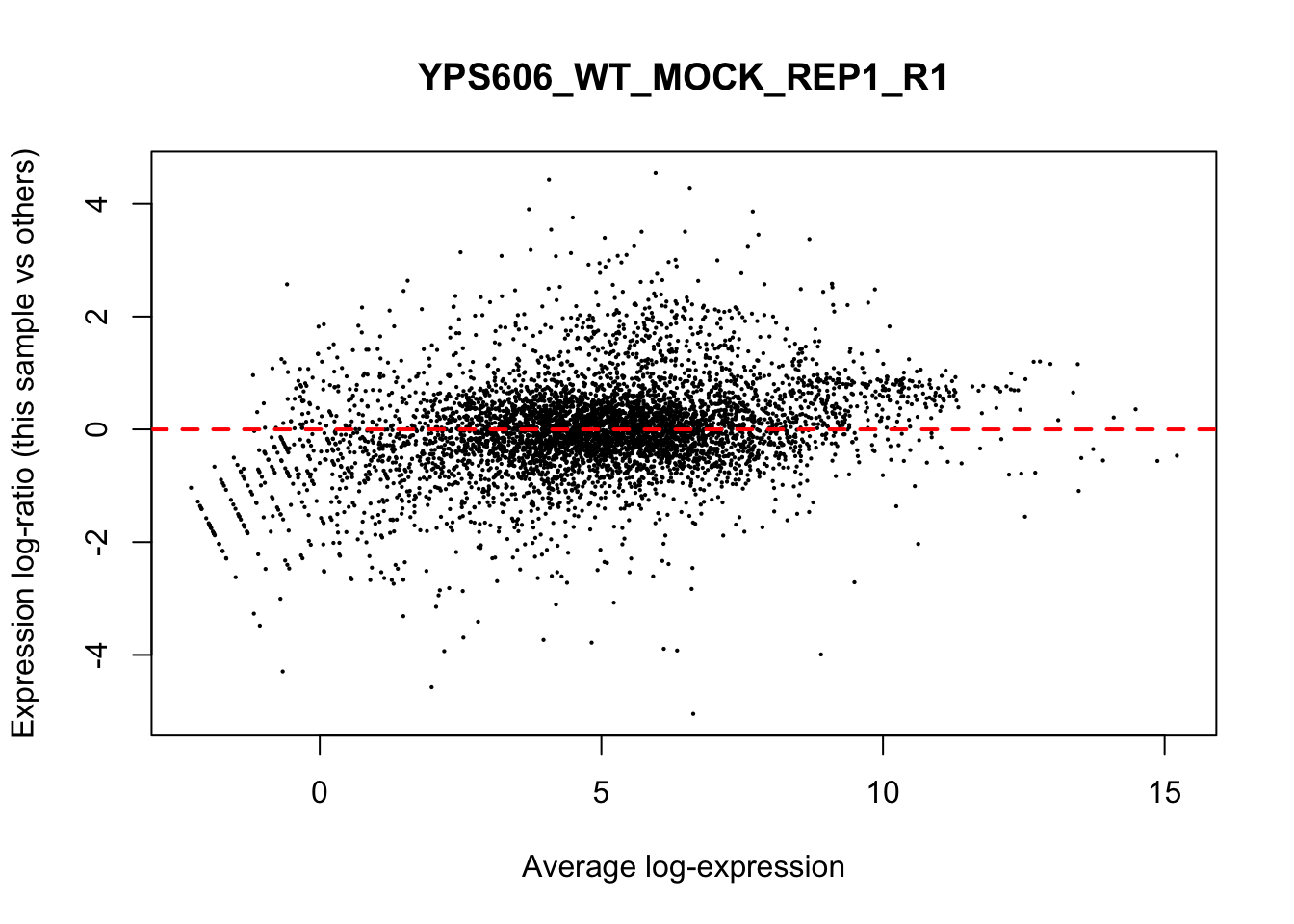
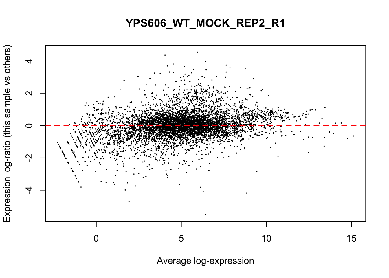
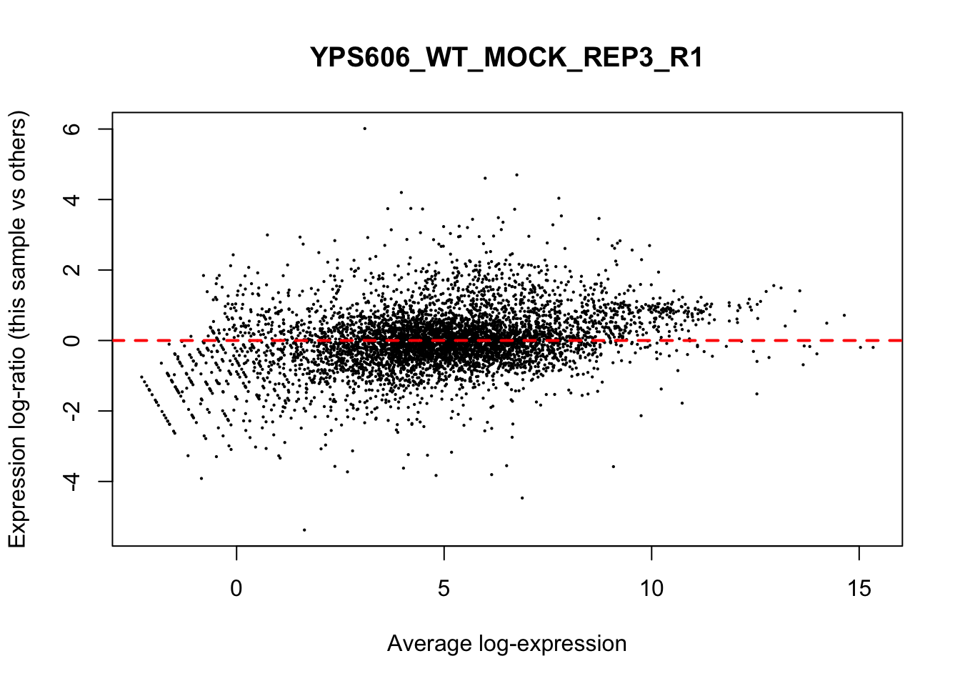
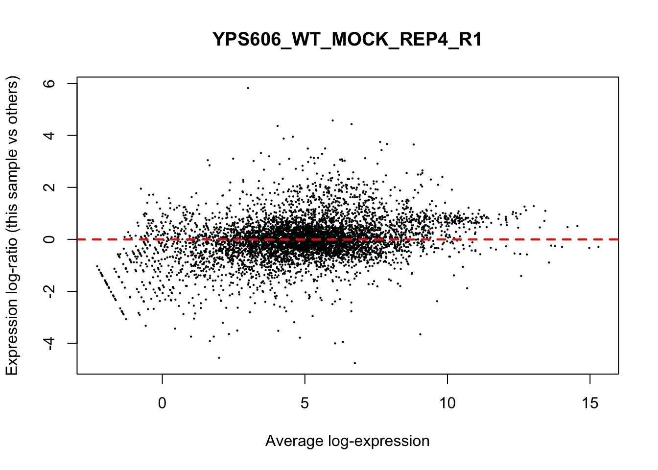
## YPS606_WT_MOCK_REP4_R1 WT.unstressed 15568155 0.951The normalization factors multiply to unity across all libraries. A normalization factor below unity indicates that the library size will be scaled down, as there is more suppression (i.e., composition bias) in that library relative to the other libraries. This is also equivalent to scaling the counts upwards in that sample. Conversely, a factor above unity scales up the library size and is equivalent to downscaling the counts. The performance of the TMM normalization procedure can be examined using mean- difference (MD) plots. This visualizes the library size-adjusted log-fold change between two libraries (the difference) against the average log-expression across those libraries (the mean). The below command plots an MD plot, comparing sample 1 against an artificial library constructed from the average of all other samples.
for (sample in 1:nrow(y$samples)) {
  plotMD(cpm(y, log=TRUE), column=sample)
  abline(h=0, col="red", lty=2, lwd=2)
}


8.7 Exploring differences between libraries
The data can be explored by generating multi-dimensional scaling (MDS) plots. This visualizes the differences between the expression profiles of different samples in two dimensions. The next plot shows the MDS plot for the yeast heatshock data.
points <- c(1,1,2,2)
colors <- rep(c("black", "red"),8)
plotMDS(y, col=colors[group], pch=points[group])
# legend("bottomright", legend=levels(group),
     # pch=points, col=colors, ncol=2)
legend("bottomright",legend=levels(group),
       pch=points, col=colors, ncol=2,
       inset=c(0,1.05), xpd=TRUE)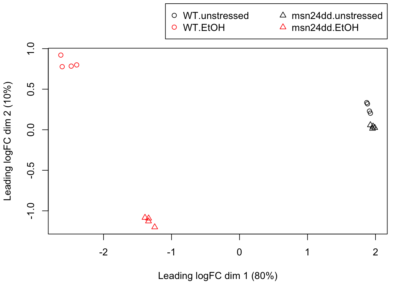
8.8 Estimate Dispersion
This is the first step in a limma analysis that differs from the edgeR workflow.
# compare this to the edgeR function estimateDisp, which uses a NB distribution.
# y <- estimateDisp(y, design, robust=TRUE)
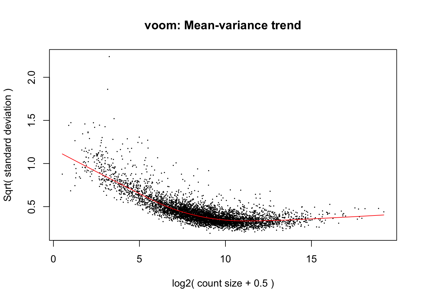
# plotBCV(y)What is voom doing?
Counts are transformed to log2 counts per million reads (CPM), where “per million reads” is defined based on the normalization factors we calculated earlier
A linear model is fitted to the log2 CPM for each gene, and the residuals are calculated
A smoothed curve is fitted to the sqrt(residual standard deviation) by average expression (see red line in plot above)
The smoothed curve is used to obtain weights for each gene and sample that are passed into limma along with the log2 CPMs.
Limma uses the lmFit function. This returns a MArrayLM object
containing the weighted least squares estimates for each gene.
##         WT.unstressed WT.EtOH msn24dd.unstressed msn24dd.EtOH
## YIL170W        -2.154   0.936             -3.239        0.851
## YFL056C         3.921   4.044              3.958        4.888
## YAR061W         0.135   0.746              0.666        0.641
## YGR014W         7.666   7.319              7.796        7.436
## YPR031W         4.711   2.735              4.857        2.818
## YIL003W         4.589   2.530              4.468        2.662
# edgeR equivalent
# fit <- glmQLFit(y, design, robust=TRUE)
# head(fit$coefficients)
# plotQLDisp(fit)Comparisons between groups (log fold-changes) are obtained as contrasts of these fitted linear models:
8.9 Testing for differential expression
The final step is to actually test for significant differential
expression in each gene, using the QL F-test. The contrast of interest
can be specified using the makeContrasts function in limma, the same
one that is used by edgeR.
# generate contrasts we are interested in learning about
my.contrasts <- makeContrasts(EtOHvsMOCK.WT = WT.EtOH - WT.unstressed,
                     EtOHvsMOCK.MSN24dd = msn24dd.EtOH - msn24dd.unstressed,
                     EtOH.MSN24ddvsWT = msn24dd.EtOH - WT.EtOH,
                     MOCK.MSN24ddvsWT = msn24dd.unstressed - WT.unstressed,
                     EtOHvsWT.MSN24ddvsWT = (msn24dd.EtOH-msn24dd.unstressed)-(WT.EtOH-WT.unstressed),
                     levels=design)

# fit the linear model to these contrasts
res_all <- contrasts.fit(fit, my.contrasts)

# This looks at all of our contrasts in my.contrasts
res_all <- eBayes(res_all)

# eBayes is the alternative to glmQLFTest in edgeR
# This contrast looks at the difference in the stress responses between mutant and WT
# res <- glmQLFTest(fit, contrast = my.contrasts)## ORF SGD GENENAME EtOHvsMOCK.WT EtOHvsMOCK.MSN24dd
## YER103W YER103W S000000905 SSA4 7.77 7.122
## YDR516C YDR516C S000002924 EMI2 7.03 3.031
## YCL040W YCL040W S000000545 GLK1 8.51 6.833
## YMR105C YMR105C S000004711 PGM2 7.62 0.792
## YLL039C YLL039C S000003962 UBI4 5.75 3.840
## YJL052W YJL052W S000003588 TDH1 10.02 9.028
## YOR317W YOR317W S000005844 FAA1 5.36 4.624
## YBL039C YBL039C S000000135 URA7 -6.93 -5.470
## YGL037C YGL037C S000003005 PNC1 6.10 3.849
## YHR104W YHR104W S000001146 GRE3 4.94 2.519
## YGR254W YGR254W S000003486 ENO1 7.83 7.590
## YBR126C YBR126C S000000330 TPS1 5.36 1.908
## YPL012W YPL012W S000005933 RRP12 -5.12 -4.315
## YDR399W YDR399W S000002807 HPT1 -5.12 -5.460
## YHR170W YHR170W S000001213 NMD3 -4.26 -3.542
## YLR258W YLR258W S000004248 GSY2 7.54 2.699
## YGR159C YGR159C S000003391 NSR1 -6.88 -5.983
## YMR196W YMR196W S000004809 <NA> 7.36 2.198
## YLL026W YLL026W S000003949 HSP104 5.70 3.659
## YML100W YML100W S000004566 TSL1 7.79 0.658
## EtOH.MSN24ddvsWT MOCK.MSN24ddvsWT EtOHvsWT.MSN24ddvsWT AveExpr F
## YER103W -0.797 -0.15215 -0.645 7.81 3407
## YDR516C -4.710 -0.71026 -4.000 6.13 2659
## YCL040W -2.077 -0.39710 -1.680 8.06 2600
## YMR105C -6.969 -0.14072 -6.829 6.08 2204
## YLL039C -2.135 -0.22780 -1.907 7.23 2067
## YJL052W -1.209 -0.22146 -0.988 8.83 2000
## YOR317W -0.979 -0.24259 -0.736 7.06 1964
## YBL039C 1.423 -0.03529 1.458 6.17 1942
## YGL037C -2.856 -0.60381 -2.252 6.60 1920
## YHR104W -2.568 -0.14350 -2.424 6.99 1910
## YGR254W -0.725 -0.48483 -0.240 10.64 1849
## YBR126C -3.646 -0.19755 -3.448 7.99 1789
## YPL012W 0.814 0.00468 0.809 6.77 1761
## YDR399W -0.422 -0.08242 -0.339 6.27 1697
## YHR170W 0.687 -0.03394 0.721 6.27 1675
## YLR258W -5.233 -0.38790 -4.845 5.01 1626
## YGR159C 0.761 -0.13994 0.901 7.21 1606
## YMR196W -4.953 0.20940 -5.162 5.42 1604
## YLL026W -1.492 0.54538 -2.038 7.84 1571
## YML100W -7.508 -0.37240 -7.136 5.91 1557
## P.Value adj.P.Val
## YER103W 3.36e-30 1.89e-26
## YDR516C 5.53e-29 1.33e-25
## YCL040W 7.11e-29 1.33e-25
## YMR105C 4.59e-28 6.45e-25
## YLL039C 9.49e-28 1.07e-24
## YJL052W 1.37e-27 1.29e-24
## YOR317W 1.68e-27 1.29e-24
## YBL039C 1.91e-27 1.29e-24
## YGL037C 2.17e-27 1.29e-24
## YHR104W 2.31e-27 1.29e-24
## YGR254W 3.32e-27 1.70e-24
## YBR126C 4.84e-27 2.27e-24
## YPL012W 5.77e-27 2.49e-24
## YDR399W 8.75e-27 3.51e-24
## YHR170W 1.01e-26 3.80e-24
## YLR258W 1.42e-26 4.97e-24
## YGR159C 1.63e-26 5.16e-24
## YMR196W 1.65e-26 5.16e-24
## YLL026W 2.08e-26 6.15e-24
## YML100W 2.31e-26 6.47e-24top.table %>%
tibble() %>%
arrange(adj.P.Val) %>%
mutate(across(where(is.numeric), signif, 3)) %>%
reactable()# edgeR equivalent below:
# let's take a quick look at the results
# topTags(res, n=10)
#
# # generate a beautiful table for the pdf/html file.
# topTags(res, n=Inf) %>% data.frame() %>%
# arrange(FDR) %>%
# mutate(logFC=round(logFC,2)) %>%
# mutate(across(where(is.numeric), signif, 3)) %>%
# reactable()# Let's see how many genes in total are significantly different in any contrast
length(which(top.table$adj.P.Val < 0.05))## [1] 4911# let's summarize this and break it down by contrast.
res_all %>%
decideTests(p.value = 0.05, lfc = 0) %>%
summary()## EtOHvsMOCK.WT EtOHvsMOCK.MSN24dd EtOH.MSN24ddvsWT MOCK.MSN24ddvsWT
## Down 2260 2145 1247 10
## NotSig 1102 1285 2920 5595
## Up 2253 2185 1448 10
## EtOHvsWT.MSN24ddvsWT
## Down 756
## NotSig 4065
## Up 794# we can save the decideTests output for graphing
decide_tests_res_all_limma <- res_all %>%
decideTests(p.value = 0.05, lfc = 0)
# Bonus: limma allows us to create a venn diagram of these contrasts
# up & downregulated genes
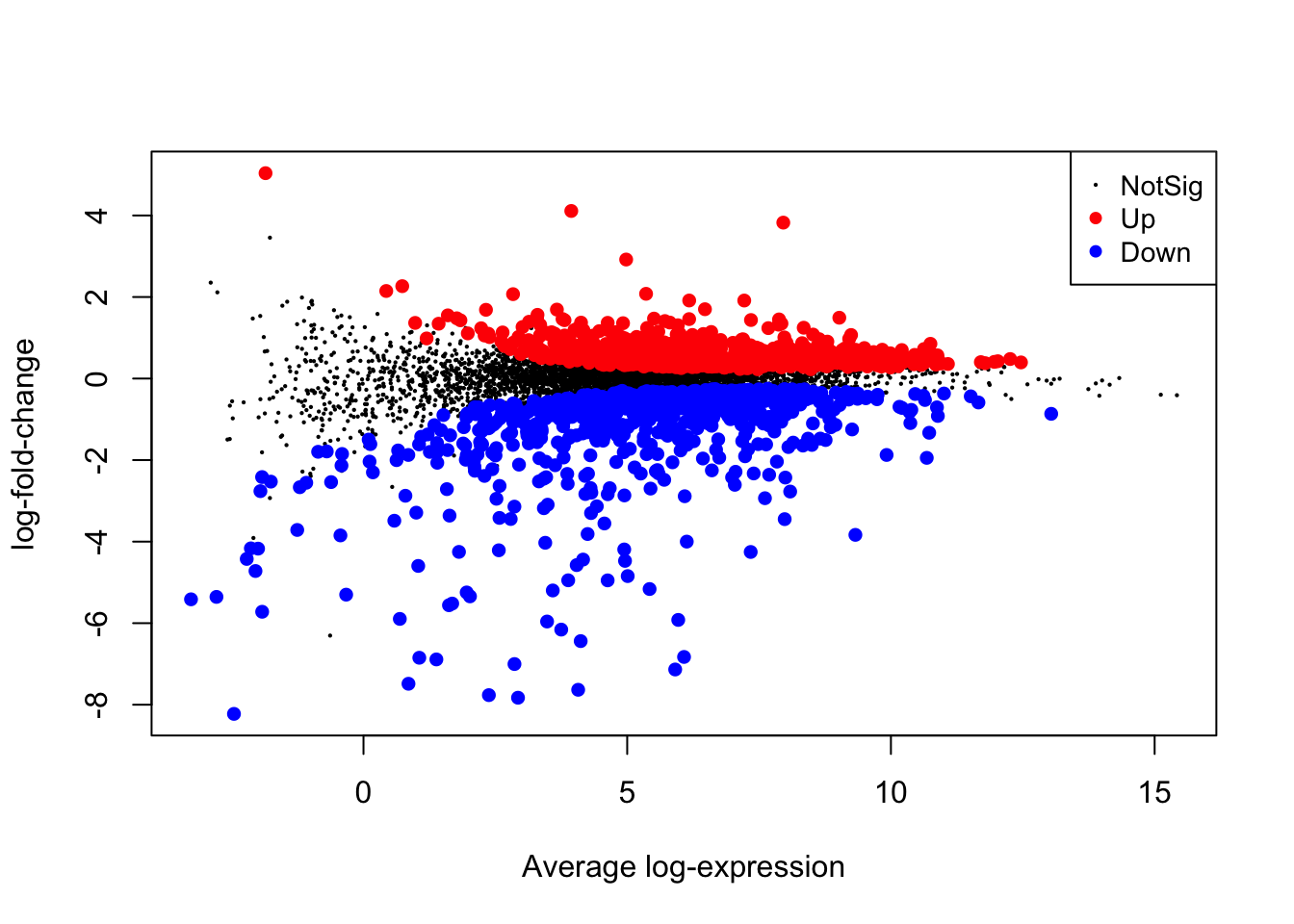
res_all %>%
decideTests(p.value = 0.05, lfc = 1) %>%
vennDiagram(include=c("up", "down"),
lwd=0.75,
mar=rep(2,4), # increase margin size
counts.col= c("red", "blue"),
show.include=TRUE)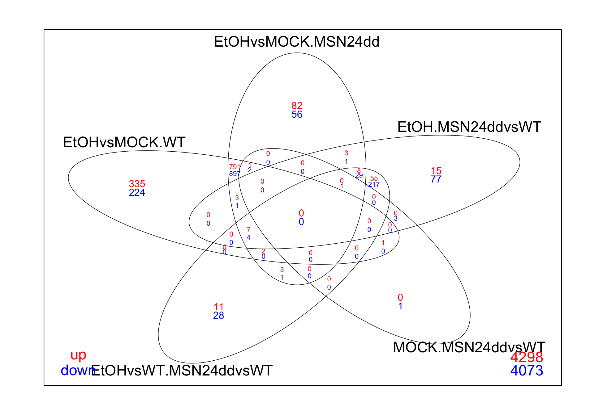
8.10 Examining a specific contrast
It is interesting to see all of the contrasts simultaneously, but often we may want to look at just a single contrast (and get the corresponding probabilities). Here is how we do that:
# fit the linear model to these contrasts
res <- contrasts.fit(fit, my.contrasts[,"EtOHvsWT.MSN24ddvsWT"])

# This contrast looks at the difference in the stress responses between mutant and WT
res <- eBayes(res)
# Note that there is no longer an "F" column, because we only look at one contrast.
top.table <- topTable(res, sort.by = "P", n = Inf)
head(top.table, 20)## ORF SGD GENENAME logFC AveExpr t P.Value adj.P.Val B
## YMR105C YMR105C S000004711 PGM2 -6.83 6.08 -39.1 2.72e-22 1.53e-18 40.3
## YKL035W YKL035W S000001518 UGP1 -3.83 9.33 -33.5 8.75e-21 2.46e-17 37.6
## YML100W YML100W S000004566 TSL1 -7.14 5.91 -32.2 2.12e-20 3.96e-17 36.3
## YBR126C YBR126C S000000330 TPS1 -3.45 7.99 -28.7 2.66e-19 3.52e-16 34.3
## YPR149W YPR149W S000006353 NCE102 -4.25 7.34 -28.5 3.13e-19 3.52e-16 34.1
## YMR196W YMR196W S000004809 <NA> -5.16 5.42 -26.4 1.70e-18 1.59e-15 32.1
## YDR516C YDR516C S000002924 EMI2 -4.00 6.13 -26.2 2.03e-18 1.63e-15 32.1
## YKL150W YKL150W S000001633 MCR1 -2.93 7.61 -25.2 4.48e-18 3.14e-15 31.5
## YPL004C YPL004C S000005925 LSP1 -2.77 8.09 -25.1 5.06e-18 3.15e-15 31.4
## YDR001C YDR001C S000002408 NTH1 -2.89 6.09 -24.6 7.76e-18 4.36e-15 31.0
## YFR053C YFR053C S000001949 HXK1 -7.63 4.07 -22.7 4.47e-17 2.28e-14 27.7
## YHR104W YHR104W S000001146 GRE3 -2.42 6.99 -21.8 1.13e-16 5.28e-14 28.3
## YER053C YER053C S000000855 PIC2 -4.95 4.63 -21.6 1.37e-16 5.68e-14 27.8
## YHL021C YHL021C S000001013 AIM17 -4.19 4.94 -21.5 1.42e-16 5.68e-14 28.0
## YLR258W YLR258W S000004248 GSY2 -4.85 5.01 -21.4 1.64e-16 6.13e-14 27.6
## YDR074W YDR074W S000002481 TPS2 -2.33 7.40 -19.6 1.11e-15 3.90e-13 26.0
## YDR258C YDR258C S000002666 HSP78 -4.47 4.96 -19.4 1.28e-15 4.24e-13 25.9
## YDR342C YDR342C S000002750 HXT7 -5.92 5.97 -18.7 2.95e-15 9.21e-13 25.1
## YGR008C YGR008C S000003240 STF2 -5.20 3.59 -17.7 9.30e-15 2.75e-12 23.2
## YGR088W YGR088W S000003320 CTT1 -6.16 3.75 -17.6 1.05e-14 2.95e-12 23.5top.table %>%
tibble() %>%
arrange(adj.P.Val) %>%
mutate(across(where(is.numeric), signif, 3)) %>%
reactable()## [,1]
## Down 756
## NotSig 4065
## Up 7948.11 Visualization
We can visualize limma results using some built-in limma functions.
8.11.1 MA lot
We need to make sure and save our output file(s).
# Choose topTags destination
dir_output_limma <-
  path.expand("~/Desktop/Genomic_Data_Analysis/Analysis/limma/")
if (!dir.exists(dir_output_limma)) {
  dir.create(dir_output_limma, recursive = TRUE)
}

# for shairng with others, the topTags output is convenient.
top.table %>% tibble() %>%
  arrange(desc(adj.P.Val)) %>%
  mutate(adj.P.Val = round(adj.P.Val, 2)) %>%
  mutate(across(where(is.numeric), signif, 3)) %>%
  write_tsv(., file = paste0(dir_output_limma, "yeast_topTags_limma.tsv"))

# for subsequent analysis, let's save the res object as an R data object.
saveRDS(object = res, file = paste0(dir_output_limma, "yeast_res_limma.Rds"))

# we might also want our y object list
saveRDS(object = y, file = paste0(dir_output_limma, "yeast_y_limma.Rds"))
8.12 treat() testing
We can use the limma command treat() to test against a fold-change
cutoff. res (or fit) can be either before or after eBayes has been
run. Note that we need to use
lfc1_res <- treat(res,
               lfc=1,
               robust = TRUE)
# treat is a limma command that can be run on fit
lfc1_top.table <- topTreat(lfc1_res, n=Inf, p.value=0.05)

# print the genes with DE significantly beyond the cutoff
lfc1_top.table
## ORF SGD GENENAME logFC AveExpr t P.Value adj.P.Val
## YMR105C YMR105C S000004711 PGM2 -6.83 6.078 -33.74 2.77e-23 1.55e-19
## YKL035W YKL035W S000001518 UGP1 -3.83 9.326 -24.66 7.44e-20 2.09e-16
## YML100W YML100W S000004566 TSL1 -7.14 5.910 -27.70 1.92e-19 3.59e-16
## YMR196W YMR196W S000004809 <NA> -5.16 5.424 -21.35 2.66e-18 3.73e-15
## YBR126C YBR126C S000000330 TPS1 -3.45 7.986 -20.39 8.23e-18 8.56e-15
## YPR149W YPR149W S000006353 NCE102 -4.25 7.342 -22.00 9.14e-18 8.56e-15
## YFR053C YFR053C S000001949 HXK1 -7.63 4.070 -19.81 1.66e-17 1.33e-14
## YDR516C YDR516C S000002924 EMI2 -4.00 6.129 -19.37 2.87e-17 2.02e-14
## YER053C YER053C S000000855 PIC2 -4.95 4.629 -17.28 4.60e-16 2.87e-13
## YLR258W YLR258W S000004248 GSY2 -4.85 5.009 -17.00 6.78e-16 3.81e-13
## YKL150W YKL150W S000001633 MCR1 -2.93 7.612 -16.69 1.05e-15 5.38e-13
## YHL021C YHL021C S000001013 AIM17 -4.19 4.944 -16.57 1.24e-15 5.80e-13
## YPL004C YPL004C S000005925 LSP1 -2.77 8.090 -16.01 2.82e-15 1.22e-12
## YDR001C YDR001C S000002408 NTH1 -2.89 6.090 -15.85 3.59e-15 1.44e-12
## YGR008C YGR008C S000003240 STF2 -5.20 3.589 -14.07 5.82e-14 2.18e-11
## YGR088W YGR088W S000003320 CTT1 -6.16 3.749 -14.84 9.98e-14 3.50e-11
## YDR258C YDR258C S000002666 HSP78 -4.47 4.959 -15.08 1.25e-13 4.13e-11
## YHR104W YHR104W S000001146 GRE3 -2.42 6.988 -12.54 7.96e-13 2.48e-10
## YMR250W YMR250W S000004862 GAD1 -4.58 4.042 -12.43 9.74e-13 2.88e-10
## YLR177W YLR177W S000004167 <NA> -3.55 4.568 -11.79 8.56e-12 2.40e-09
## YHR087W YHR087W S000001129 RTC3 -7.76 2.377 -11.68 1.03e-11 2.66e-09
## YDR074W YDR074W S000002481 TPS2 -2.33 7.398 -11.16 1.04e-11 2.66e-09
## YBR085C-A YBR085C-A S000007522 <NA> -2.84 4.630 -10.87 1.82e-11 4.45e-09
## YBR072W YBR072W S000000276 HSP26 -4.95 3.882 -10.69 2.60e-11 6.08e-09
## YFR015C YFR015C S000001911 GSY1 -5.96 3.481 -11.00 3.50e-11 7.86e-09
## YER067W YER067W S000000869 RGI1 -6.44 4.118 -11.22 4.78e-11 1.03e-08
## YGR248W YGR248W S000003480 SOL4 -6.89 1.382 -10.00 1.07e-10 2.22e-08
## YDR033W YDR033W S000002440 MRH1 -2.61 7.040 -10.66 1.14e-10 2.29e-08
## YBL064C YBL064C S000000160 PRX1 -2.32 5.593 -9.75 1.79e-10 3.47e-08
## YPR160W YPR160W S000006364 GPH1 -7.00 2.863 -10.55 2.20e-10 4.12e-08
## YOR315W YOR315W S000005842 SFG1 4.11 3.940 9.63 2.32e-10 4.21e-08
## YMR090W YMR090W S000004696 <NA> -3.30 4.314 -9.61 2.44e-10 4.28e-08
## YMR031C YMR031C S000004633 EIS1 -2.70 5.442 -9.74 6.30e-10 1.07e-07
## YFR052C-A YFR052C-A S000028768 <NA> -6.85 1.058 -8.95 1.02e-09 1.68e-07
## YEL011W YEL011W S000000737 GLC3 -4.44 4.163 -10.05 1.17e-09 1.87e-07
## YML054C YML054C S000004518 CYB2 -2.80 4.320 -8.70 1.80e-09 2.81e-07
## YBR183W YBR183W S000000387 YPC1 -4.21 2.566 -8.54 2.54e-09 3.85e-07
## YGL037C YGL037C S000003005 PNC1 -2.25 6.605 -8.41 3.41e-09 5.04e-07
## YNL007C YNL007C S000004952 SIS1 -2.29 7.054 -8.82 3.83e-09 5.51e-07
## YEL039C YEL039C S000000765 CYC7 -5.25 1.956 -8.27 4.75e-09 6.67e-07
## YDL124W YDL124W S000002282 <NA> -2.87 4.947 -8.12 6.69e-09 9.16e-07
## YDR342C YDR342C S000002750 HXT7 -5.92 5.968 -12.31 8.67e-09 1.16e-06
## YMR173W YMR173W S000004784 DDR48 -3.18 3.420 -7.99 9.06e-09 1.16e-06
## YFL014W YFL014W S000001880 HSP12 -7.83 2.930 -9.85 9.08e-09 1.16e-06
## YPL240C YPL240C S000006161 HSP82 -2.36 7.691 -8.39 1.22e-08 1.52e-06
## YOL052C-A YOL052C-A S000005413 DDR2 -8.22 -2.456 -7.76 1.57e-08 1.91e-06
## YFR017C YFR017C S000001913 IGD1 -5.56 1.621 -7.75 2.04e-08 2.44e-06
## YML128C YML128C S000004597 MSC1 -2.39 4.202 -7.55 2.57e-08 3.01e-06
## YLL026W YLL026W S000003949 HSP104 -2.04 7.838 -7.54 2.63e-08 3.02e-06
## YLR178C YLR178C S000004168 TFS1 -2.83 4.206 -7.53 3.22e-08 3.62e-06
## YLR152C YLR152C S000004142 <NA> -2.42 3.464 -7.40 3.69e-08 4.06e-06
## YMR261C YMR261C S000004874 TPS3 -1.74 7.291 -7.13 7.15e-08 7.72e-06
## YGR070W YGR070W S000003302 ROM1 -2.34 3.863 -7.10 7.65e-08 7.98e-06
## YMR169C YMR169C S000004779 ALD3 -4.03 3.446 -7.79 7.68e-08 7.98e-06
## YLL039C YLL039C S000003962 UBI4 -1.91 7.235 -6.99 1.01e-07 1.03e-05
## YCR091W YCR091W S000000687 KIN82 -2.46 3.418 -6.98 1.03e-07 1.03e-05
## YOR161C YOR161C S000005687 PNS1 -3.81 4.249 -8.20 1.07e-07 1.06e-05
## YKL151C YKL151C S000001634 NNR2 -2.25 5.572 -6.95 1.13e-07 1.09e-05
## YBL075C YBL075C S000000171 SSA3 -1.86 5.368 -6.75 1.84e-07 1.75e-05
## YJL042W YJL042W S000003578 MHP1 -1.76 6.012 -6.55 3.00e-07 2.81e-05
## YNL160W YNL160W S000005104 YGP1 -2.69 4.669 -6.71 3.36e-07 3.09e-05
## YNR034W-A YNR034W-A S000007525 EGO4 -7.49 0.853 -6.55 5.60e-07 5.08e-05
## YDL204W YDL204W S000002363 RTN2 -3.44 2.791 -6.31 6.20e-07 5.53e-05
## YBL015W YBL015W S000000111 ACH1 -2.05 5.858 -6.34 7.13e-07 6.26e-05
## YBR169C YBR169C S000000373 SSE2 -2.69 4.305 -6.15 8.37e-07 7.23e-05
## YPL230W YPL230W S000006151 USV1 -4.25 1.810 -6.11 1.43e-06 1.22e-04
## YBR230C YBR230C S000000434 OM14 -2.33 5.257 -6.31 1.51e-06 1.27e-04
## YFL051C YFL051C S000001843 <NA> 2.92 4.980 6.49 1.81e-06 1.49e-04
## YNL015W YNL015W S000004960 PBI2 -2.58 3.872 -5.80 2.17e-06 1.77e-04
## YOR298C-A YOR298C-A S000007253 MBF1 -1.61 7.482 -5.58 3.65e-06 2.92e-04
## YNL274C YNL274C S000005218 GOR1 -2.52 3.327 -5.56 3.84e-06 3.04e-04
## YBR214W YBR214W S000000418 SDS24 -2.27 5.543 -5.56 3.93e-06 3.07e-04
## YDR277C YDR277C S000002685 MTH1 -2.63 2.580 -5.43 5.36e-06 4.13e-04
## YGR281W YGR281W S000003513 YOR1 -1.53 7.181 -5.39 6.05e-06 4.56e-04
## YOR173W YOR173W S000005699 DCS2 -2.95 2.521 -5.39 6.09e-06 4.56e-04
## YER073W YER073W S000000875 ALD5 1.91 6.175 5.54 6.59e-06 4.87e-04
## YBR149W YBR149W S000000353 ARA1 -1.62 7.634 -5.32 7.18e-06 5.24e-04
## YLL023C YLL023C S000003946 POM33 -1.96 6.435 -5.60 8.36e-06 6.02e-04
## YOR347C YOR347C S000005874 PYK2 -3.42 2.578 -5.24 9.04e-06 6.43e-04
## YLR327C YLR327C S000004319 TMA10 -5.90 0.689 -5.23 1.37e-05 9.55e-04
## YOR052C YOR052C S000005578 TMC1 -1.94 3.794 -5.08 1.38e-05 9.55e-04
## YGR019W YGR019W S000003251 UGA1 -1.81 4.934 -5.02 1.61e-05 1.10e-03
## YDL039C YDL039C S000002197 PRM7 2.08 5.358 5.25 1.74e-05 1.18e-03
## YDL181W YDL181W S000002340 INH1 -1.62 5.447 -4.86 2.42e-05 1.62e-03
## YKL037W YKL037W S000001520 AIM26 -5.72 -1.921 -4.83 2.68e-05 1.77e-03
## YDR216W YDR216W S000002624 ADR1 -2.13 3.634 -4.81 2.76e-05 1.80e-03
## YGR086C YGR086C S000003318 PIL1 -1.51 8.762 -4.78 2.98e-05 1.92e-03
## YER066C-A YER066C-A S000002959 <NA> -5.36 -2.787 -4.77 3.07e-05 1.96e-03
## YDR275W YDR275W S000002683 BSC2 -2.22 2.441 -4.74 3.32e-05 2.10e-03
## YHR092C YHR092C S000001134 HXT4 -3.09 3.492 -5.14 3.54e-05 2.21e-03
## YDR533C YDR533C S000002941 HSP31 -2.04 3.459 -4.71 3.64e-05 2.25e-03
## YMR145C YMR145C S000004753 NDE1 -1.57 8.147 -4.68 3.89e-05 2.37e-03
## YNL194C YNL194C S000005138 <NA> -5.30 -0.328 -4.69 4.03e-05 2.43e-03
## YIL056W YIL056W S000001318 VHR1 -1.63 5.441 -4.67 4.07e-05 2.43e-03
## YPL014W YPL014W S000005935 CIP1 -2.05 4.793 -4.77 5.47e-05 3.23e-03
## YAL065C YAL065C S000001817 <NA> 5.04 -1.857 4.53 5.80e-05 3.39e-03
## YKL201C YKL201C S000001684 MNN4 -2.18 5.141 -4.91 6.06e-05 3.51e-03
## YJL141C YJL141C S000003677 YAK1 -1.72 5.050 -4.50 6.27e-05 3.59e-03
## YPL061W YPL061W S000005982 ALD6 3.82 7.959 5.49 6.35e-05 3.60e-03
## YAL060W YAL060W S000000056 BDH1 -1.94 6.745 -4.87 6.51e-05 3.65e-03
## YBR117C YBR117C S000000321 TKL2 -3.36 1.632 -4.57 6.90e-05 3.84e-03
## YDR185C YDR185C S000002593 UPS3 -2.26 2.111 -4.41 7.95e-05 4.37e-03
## YNR014W YNR014W S000005297 <NA> -5.52 1.682 -4.93 8.81e-05 4.80e-03
## YER054C YER054C S000000856 GIP2 -3.49 0.585 -4.36 9.10e-05 4.92e-03
## YDR513W YDR513W S000002921 GRX2 -1.49 6.726 -4.25 1.20e-04 6.43e-03
## YER067C-A YER067C-A S000028748 <NA> -5.41 -3.270 -4.21 1.38e-04 7.24e-03
## YIL136W YIL136W S000001398 OM45 -2.39 2.294 -4.20 1.38e-04 7.24e-03
## YPR184W YPR184W S000006388 GDB1 -1.85 5.573 -4.24 1.57e-04 8.16e-03
## YMR251W-A YMR251W-A S000004864 HOR7 -3.13 4.424 -4.60 1.60e-04 8.22e-03
## YOL155C YOL155C S000005515 HPF1 -1.87 9.918 -4.41 1.72e-04 8.78e-03
## YBR139W YBR139W S000000343 <NA> -1.62 6.133 -4.06 1.98e-04 1.00e-02
## YOR185C YOR185C S000005711 GSP2 -1.88 4.302 -4.00 2.33e-04 1.17e-02
## YBR161W YBR161W S000000365 CSH1 -1.69 3.783 -3.96 2.59e-04 1.29e-02
## YBR054W YBR054W S000000258 YRO2 -4.60 1.038 -4.14 2.61e-04 1.29e-02
## YBL049W YBL049W S000000145 MOH1 -4.72 -2.048 -3.92 2.90e-04 1.42e-02
## YOR345C YOR345C S000005872 <NA> -4.42 -2.214 -3.91 2.98e-04 1.44e-02
## YDR345C YDR345C S000002753 HXT3 -2.43 7.998 -4.45 3.27e-04 1.56e-02
## YCL040W YCL040W S000000545 GLK1 -1.68 8.056 -3.87 3.29e-04 1.56e-02
## YAL005C YAL005C S000000004 SSA1 -1.94 10.680 -4.16 3.44e-04 1.62e-02
## YJL107C YJL107C S000003643 <NA> -1.89 2.503 -3.83 3.60e-04 1.68e-02
## YCR021C YCR021C S000000615 HSP30 -5.34 2.019 -4.31 3.70e-04 1.72e-02
## YMR081C YMR081C S000004686 ISF1 -3.85 -0.437 -3.81 3.86e-04 1.78e-02
## YKL096W YKL096W S000001579 CWP1 -2.48 5.702 -4.24 4.91e-04 2.24e-02
## YGR143W YGR143W S000003375 SKN1 -1.52 4.422 -3.64 6.00e-04 2.71e-02
## YDL022W YDL022W S000002180 GPD1 -1.64 8.332 -3.65 8.10e-04 3.64e-02
## YKR049C YKR049C S000001757 FMP46 -2.16 2.104 -3.50 8.54e-04 3.78e-02
## YNL200C YNL200C S000005144 NNR1 -2.11 2.949 -3.50 8.56e-04 3.78e-02
## YNL195C YNL195C S000005139 <NA> -3.29 1.001 -3.45 9.91e-04 4.35e-02
## YCL035C YCL035C S000000540 GRX1 -1.54 5.312 -3.43 1.00e-03 4.37e-02
## YPL087W YPL087W S000006008 YDC1 -1.54 6.261 -3.44 1.06e-03 4.60e-02
## YOR374W YOR374W S000005901 ALD4 -1.75 6.685 -3.58 1.09e-03 4.65e-02
## YPR026W YPR026W S000006230 ATH1 -1.51 4.864 -3.37 1.18e-03 4.97e-02
## YMR016C YMR016C S000004618 SOK2 1.47 5.508 3.37 1.18e-03 4.97e-02# for subsequent analysis, let's save the output file as a tsv
# and the res object as an R data object.
lfc1_top.table %>% tibble() %>%
arrange(desc(adj.P.Val)) %>%
mutate(adj.P.Val = round(adj.P.Val, 2)) %>%
mutate(across(where(is.numeric), signif, 3)) %>%
write_tsv(., file = paste0(dir_output_limma, "yeast_lfc1_topTreat_limma.tsv"))
saveRDS(object = lfc1_res, file = paste0(dir_output_limma, "yeast_lfc1_res_limma.Rds"))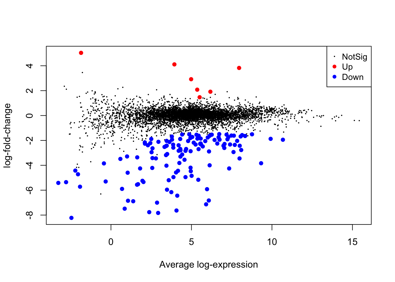
8.13 Comparing DE analysis softwares
We have went through some example DE workflows with edgeR, DESeq2, and limma-voom. Since we have saved our outputs for each analysis, we can compare their outcomes now.
# load in all of the DE results for the difference of difference contrast
path_output_edgeR <- "~/Desktop/Genomic_Data_Analysis/Analysis/edgeR/yeast_topTags_edgeR.tsv"
path_output_DESeq2 <- "~/Desktop/Genomic_Data_Analysis/Analysis/DESeq2/yeast_res_DESeq2.tsv"
path_output_limma <- "~/Desktop/Genomic_Data_Analysis/Analysis/limma/yeast_topTags_limma.tsv"

topTags_edgeR <- read.delim(path_output_edgeR)
topTags_DESeq2 <- read.delim(path_output_DESeq2)
topTags_limma <- read.delim(path_output_limma)
sig_cutoff <- 0.01
FC_cutoff <- 1
# NOTE: we need to be very careful applying an FC cutoff like this
## edgeR
# get genes that are upregualted
up_edgeR_DEG <- topTags_edgeR %>%
dplyr::filter(FDR < sig_cutoff & logFC > FC_cutoff) %>%
pull(ORF)
down_edgeR_DEG <- topTags_edgeR %>%
dplyr::filter(FDR < sig_cutoff & logFC < -FC_cutoff) %>%
pull(ORF)
## DESeq2
up_DESeq2_DEG <- topTags_DESeq2 %>%
dplyr::filter(padj < sig_cutoff & log2FoldChange > FC_cutoff) %>%
pull(ORF)
down_DESeq2_DEG <- topTags_DESeq2 %>%
dplyr::filter(padj < sig_cutoff & log2FoldChange < -FC_cutoff) %>%
pull(ORF)
## limma
up_limma_DEG <- topTags_limma %>%
dplyr::filter(adj.P.Val < sig_cutoff & logFC > FC_cutoff) %>%
pull(ORF)
down_limma_DEG <- topTags_limma %>%
dplyr::filter(adj.P.Val < sig_cutoff & logFC < -FC_cutoff) %>%
pull(ORF)
up_DEG_results_list <- list(up_edgeR_DEG,
up_DESeq2_DEG,
up_limma_DEG)
# visualize the GO results list as a venn diagram
ggVennDiagram(up_DEG_results_list,
category.names = c("edgeR", "DESeq2", "limma")) +
scale_x_continuous(expand = expansion(mult = .2)) +
scale_fill_distiller(palette = "RdBu"
) +
ggtitle("Upregulated genes in contrast: \n(EtOH.MSN2/4dd - MOCK.MSN2/4dd) - (EtOH.WT - MOCK.WT)")
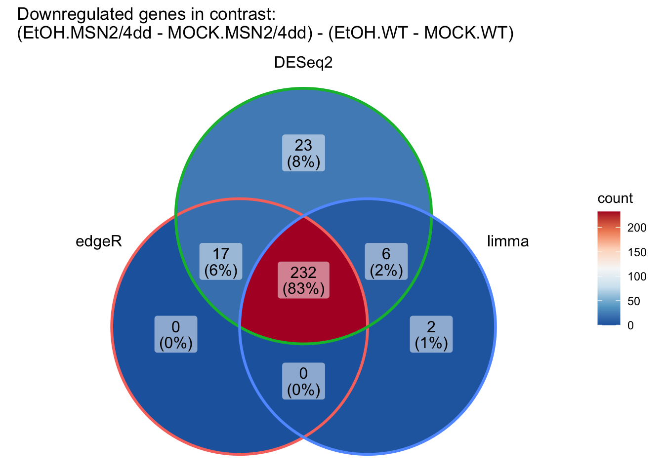
# Now let's do the same for downregulated genes:
down_DEG_results_list <- list(down_edgeR_DEG,
down_DESeq2_DEG,
down_limma_DEG)
ggVennDiagram(down_DEG_results_list,
category.names = c("edgeR", "DESeq2", "limma")) +
scale_x_continuous(expand = expansion(mult = .2)) +
scale_fill_distiller(palette = "RdBu"
) +
ggtitle("Downregulated genes in contrast: \n(EtOH.MSN2/4dd - MOCK.MSN2/4dd) - (EtOH.WT - MOCK.WT)")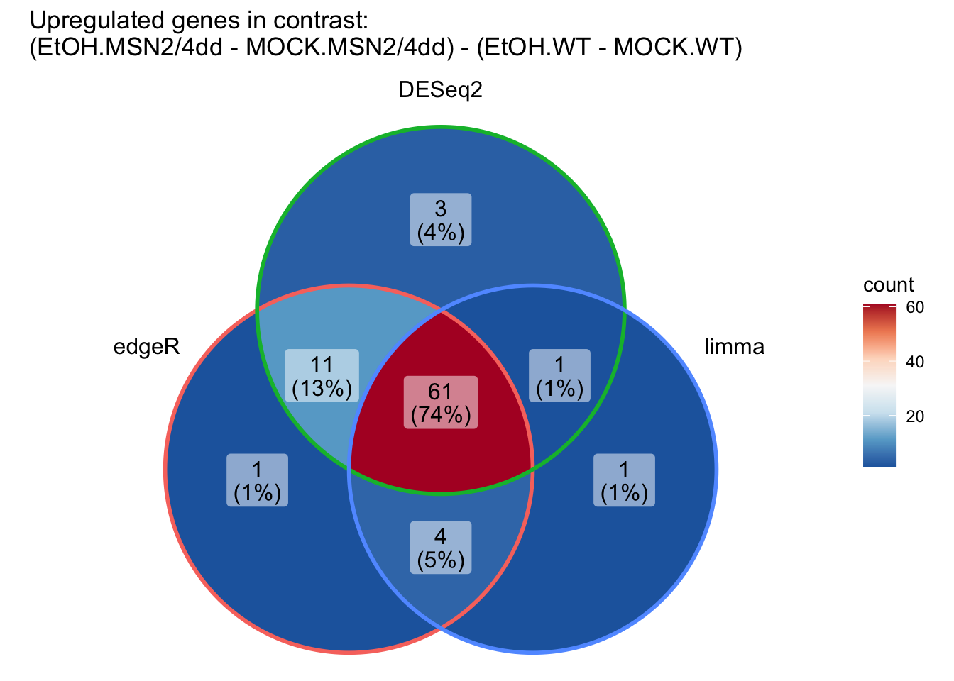
8.14 Correlation between logFC estimates across softwares
# Custom labels for facet headers
custom_labels <- c("purple" = "Sig in Both",
                   "red" = "Only in edgeR",
                   "blue" = "Only in DESeq2",
                   "black" = "Not Sig",
                   "grey" = "NA encountered")


# compare edgeR & DESeq2
full_join(topTags_edgeR, topTags_DESeq2,
          by = join_by(ORF, SGD, GENENAME)) %>%
  mutate(edgeR_sig = ifelse(FDR < sig_cutoff, "red", "black")) %>%
  mutate(DESeq2_sig = ifelse(padj < sig_cutoff, "blue", "black")) %>%
  mutate(sig = factor(case_when(
    edgeR_sig == "red" & DESeq2_sig == "blue" ~ "purple",
    edgeR_sig == "red" & DESeq2_sig != "blue" ~ "red",
    edgeR_sig != "red" & DESeq2_sig == "blue" ~ "blue",
    edgeR_sig != "red" & DESeq2_sig != "blue" ~ "black",
    TRUE ~ "grey"  # if none of these are met
  ), levels = c("purple", "red", "blue", "black", "grey"), labels = c("Sig in Both", "Only in edgeR", "Only in DESeq2", "Not Sig", "NA encountered"))) %>%
  ggplot(aes(x=logFC, y=log2FoldChange, color = sig, size=logCPM)) +
  geom_abline(slope = 1,) +
  geom_point(alpha=0.5) +
  scale_color_manual(values=c("purple", "red", "blue", "black", "grey")) + # use colors given
  theme_bw() +
  facet_wrap(~sig, labeller = labeller(new_column = custom_labels)) +
  ggtitle("Comparing genewise logFC estimates between edgeR and DESeq2")
## Warning: Removed 11 rows containing missing values (`geom_point()`).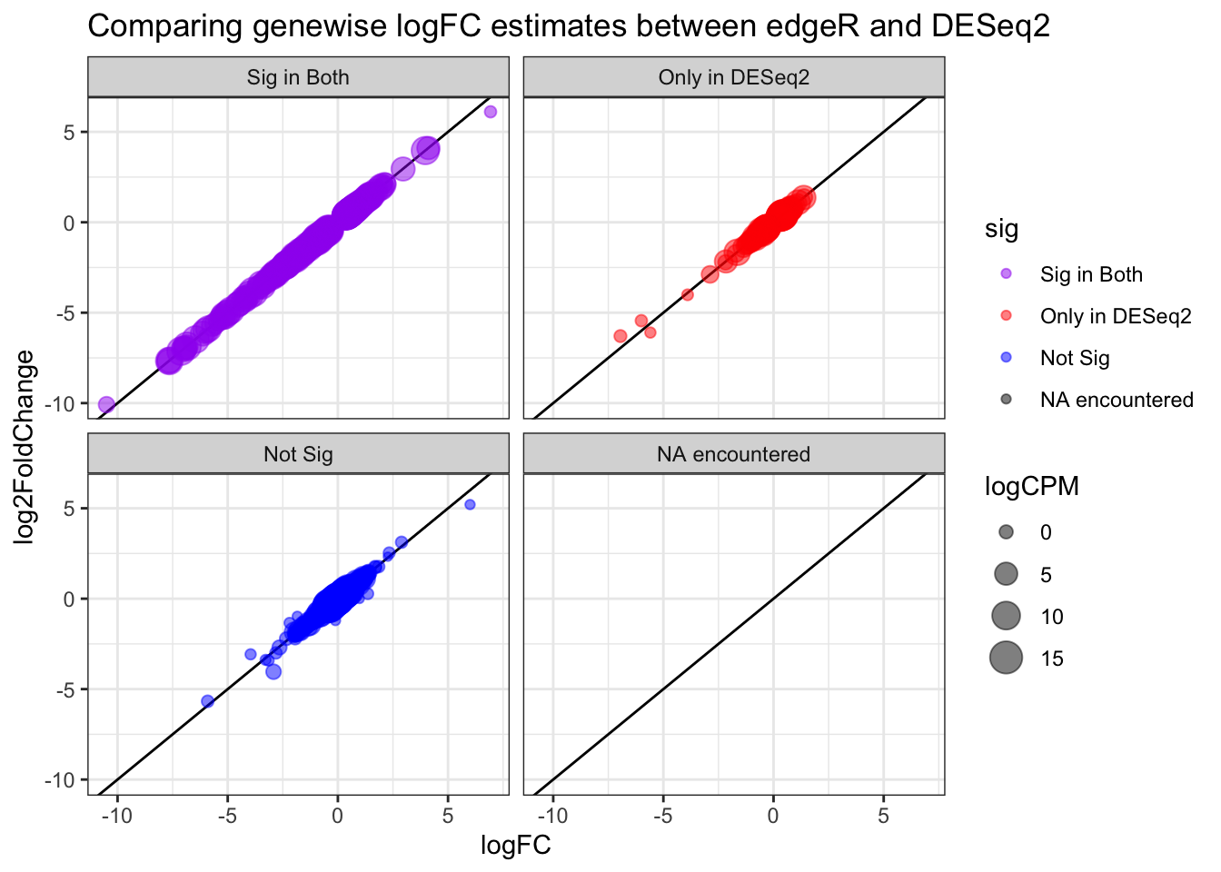
# compare edgeR & limma
full_join(topTags_edgeR, topTags_limma,
          by = join_by(ORF, SGD, GENENAME)) %>%
  mutate(edgeR_sig = ifelse(FDR < sig_cutoff, "red", "black")) %>%
  mutate(limma_sig = ifelse(adj.P.Val < sig_cutoff, "green", "black")) %>%
  mutate(sig = factor(case_when(
    edgeR_sig == "red" & limma_sig == "green" ~ "brown",
    edgeR_sig == "red" & limma_sig != "green" ~ "red",
    edgeR_sig != "red" & limma_sig == "green" ~ "green",
    edgeR_sig != "red" & limma_sig != "green" ~ "black",
    TRUE ~ "grey"  # if none of these are met
  ), levels = c("brown", "red", "green", "black", "grey"), labels = c("Sig in Both", "Only in edgeR", "Only in limma", "Not Sig", "NA encountered"))) %>%
  ggplot(aes(x=logFC.x, y=logFC.y, color = sig, size=logCPM)) +
  geom_abline(slope = 1,) +
  geom_point(alpha=0.5) +
  scale_color_manual(values=c("brown", "red", "green", "black", "grey")) + # use colors given
  theme_bw() +
  facet_wrap(~sig, labeller = labeller(new_column = custom_labels)) +
  ggtitle("Comparing genewise logFC estimates between edgeR and limma") +
  labs(x="logFC estimate: edgeR", y="logFC estimate: limma")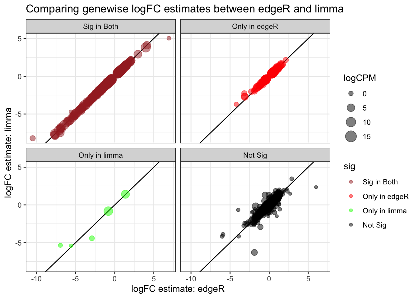
# compare DESeq2 & limma
full_join(topTags_DESeq2, topTags_limma,
          by = join_by(ORF, SGD, GENENAME)) %>%
  mutate(DESeq2_sig = ifelse(padj < sig_cutoff, "blue", "black")) %>%
  mutate(limma_sig = ifelse(adj.P.Val < sig_cutoff, "green", "black")) %>%
  mutate(sig = factor(case_when(
    DESeq2_sig == "blue" & limma_sig == "green" ~ "aquamarine3",
    DESeq2_sig == "blue" & limma_sig != "green" ~ "blue",
    DESeq2_sig != "blue" & limma_sig == "green" ~ "green",
    DESeq2_sig != "blue" & limma_sig != "green" ~ "black",
    TRUE ~ "grey"  # if none of these are met
  ), levels = c("aquamarine3", "blue", "green", "black", "grey"), labels = c("Sig in Both", "Only in DESeq2", "Only in limma", "Not Sig", "NA encountered"))) %>%
  ggplot(aes(x=log2FoldChange, y=logFC, color = sig, size=AveExpr)) +
  geom_abline(slope = 1,) +
  geom_point(alpha=0.5) +
  scale_color_manual(values=c("aquamarine3", "blue", "green", "black", "grey")) + # use colors given
  theme_bw() +
  facet_wrap(~sig, labeller = labeller(new_column = custom_labels, drop=FALSE)) +
  ggtitle("Comparing genewise logFC estimates between DESeq2 and limma") +
  labs(x="logFC estimate: DESeq2", y="logFC estimate: limma")
## Warning: Removed 11 rows containing missing values (`geom_point()`).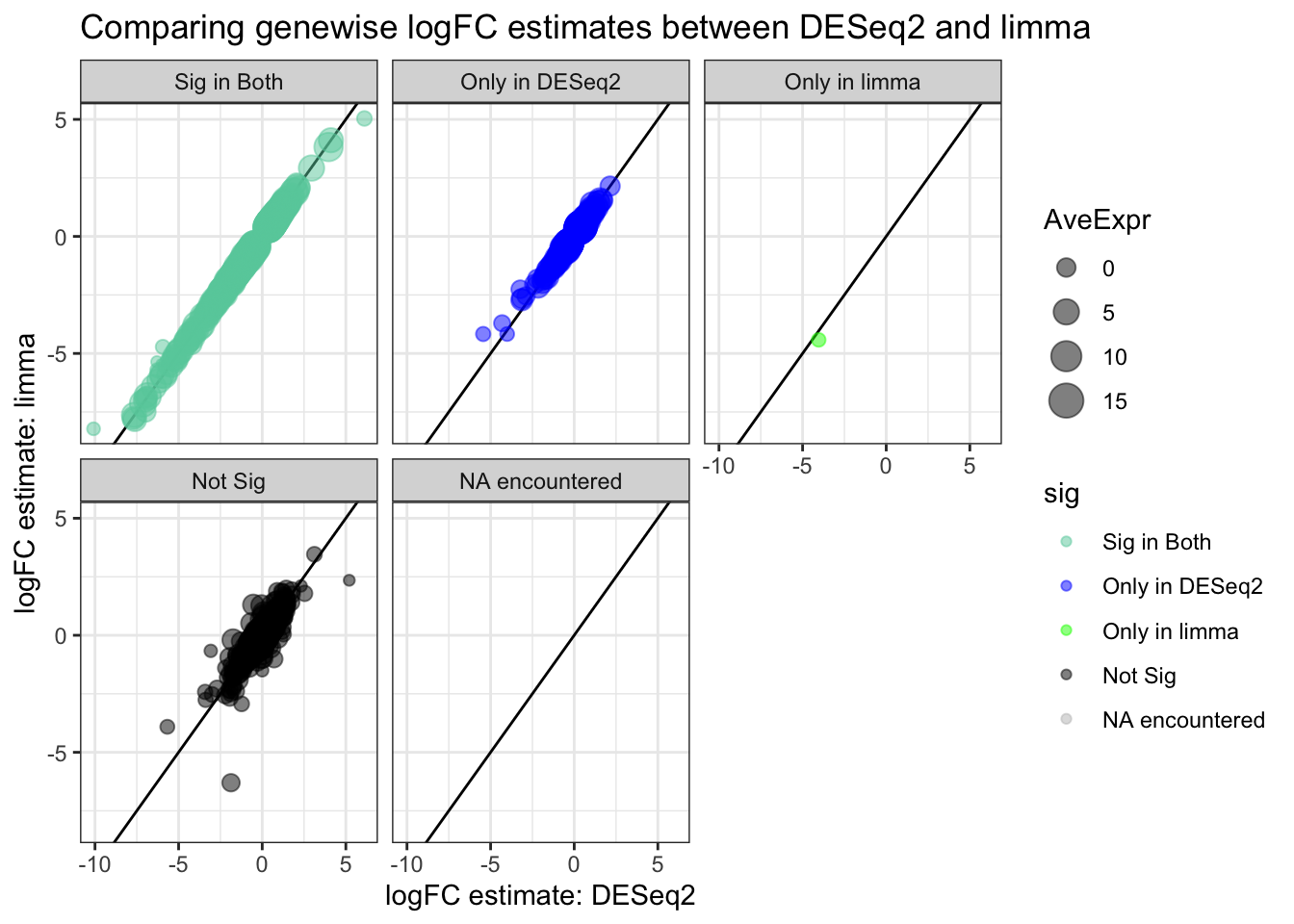
8.15 Questions
Question 1: How many genes were upregulated and downregulated in the contrast we looked at in today’s activity? Be sure to clarify the cutoffs used for determining significance.
Question 2: What are the pros and cons of applying a logFC cutoff to a differential expression analysis?
Be sure to knit this file into a pdf or html file once you’re finished.
System information for reproducibility:
R version 4.3.1 (2023-06-16)
Platform: aarch64-apple-darwin20 (64-bit)
locale: en_US.UTF-8||en_US.UTF-8||en_US.UTF-8||C||en_US.UTF-8||en_US.UTF-8
attached base packages: stats4, stats, graphics, grDevices, utils, datasets, methods and base
other attached packages: Glimma(v.2.10.0), DESeq2(v.1.40.2), edgeR(v.3.42.4), limma(v.3.56.2), reactable(v.0.4.4), webshot2(v.0.1.1), statmod(v.1.5.0), Rsubread(v.2.14.2), ShortRead(v.1.58.0), GenomicAlignments(v.1.36.0), SummarizedExperiment(v.1.30.2), MatrixGenerics(v.1.12.3), matrixStats(v.1.0.0), Rsamtools(v.2.16.0), GenomicRanges(v.1.52.1), Biostrings(v.2.68.1), GenomeInfoDb(v.1.36.4), XVector(v.0.40.0), BiocParallel(v.1.34.2), Rfastp(v.1.10.0), org.Sc.sgd.db(v.3.17.0), AnnotationDbi(v.1.62.2), IRanges(v.2.34.1), S4Vectors(v.0.38.2), Biobase(v.2.60.0), BiocGenerics(v.0.46.0), clusterProfiler(v.4.8.2), ggVennDiagram(v.1.2.3), tidytree(v.0.4.5), igraph(v.1.5.1), janitor(v.2.2.0), BiocManager(v.1.30.22), pander(v.0.6.5), knitr(v.1.44), here(v.1.0.1), lubridate(v.1.9.3), forcats(v.1.0.0), stringr(v.1.5.0), dplyr(v.1.1.3), purrr(v.1.0.2), readr(v.2.1.4), tidyr(v.1.3.0), tibble(v.3.2.1), ggplot2(v.3.4.4), tidyverse(v.2.0.0) and pacman(v.0.5.1)
loaded via a namespace (and not attached): splines(v.4.3.1), later(v.1.3.1), bitops(v.1.0-7), ggplotify(v.0.1.2), polyclip(v.1.10-6), lifecycle(v.1.0.3), sf(v.1.0-14), rprojroot(v.2.0.3), vroom(v.1.6.4), processx(v.3.8.2), lattice(v.0.21-9), MASS(v.7.3-60), crosstalk(v.1.2.0), magrittr(v.2.0.3), sass(v.0.4.7), rmarkdown(v.2.25), jquerylib(v.0.1.4), yaml(v.2.3.7), cowplot(v.1.1.1), chromote(v.0.1.2), DBI(v.1.1.3), RColorBrewer(v.1.1-3), abind(v.1.4-5), zlibbioc(v.1.46.0), ggraph(v.2.1.0), RCurl(v.1.98-1.12), yulab.utils(v.0.1.0), tweenr(v.2.0.2), GenomeInfoDbData(v.1.2.10), enrichplot(v.1.20.0), ggrepel(v.0.9.4), units(v.0.8-4), codetools(v.0.2-19), DelayedArray(v.0.26.7), DOSE(v.3.26.1), ggforce(v.0.4.1), tidyselect(v.1.2.0), aplot(v.0.2.2), farver(v.2.1.1), viridis(v.0.6.4), jsonlite(v.1.8.7), e1071(v.1.7-13), ellipsis(v.0.3.2), tidygraph(v.1.2.3), tools(v.4.3.1), treeio(v.1.24.3), Rcpp(v.1.0.11), glue(v.1.6.2), gridExtra(v.2.3), xfun(v.0.40), qvalue(v.2.32.0), websocket(v.1.4.1), withr(v.2.5.1), fastmap(v.1.1.1), latticeExtra(v.0.6-30), fansi(v.1.0.5), digest(v.0.6.33), timechange(v.0.2.0), R6(v.2.5.1), gridGraphics(v.0.5-1), colorspace(v.2.1-0), GO.db(v.3.17.0), jpeg(v.0.1-10), RSQLite(v.2.3.1), utf8(v.1.2.3), generics(v.0.1.3), data.table(v.1.14.8), class(v.7.3-22), graphlayouts(v.1.0.1), httr(v.1.4.7), htmlwidgets(v.1.6.2), S4Arrays(v.1.0.6), scatterpie(v.0.2.1), pkgconfig(v.2.0.3), gtable(v.0.3.4), blob(v.1.2.4), hwriter(v.1.3.2.1), shadowtext(v.0.1.2), htmltools(v.0.5.6.1), bookdown(v.0.36), fgsea(v.1.26.0), scales(v.1.2.1), png(v.0.1-8), snakecase(v.0.11.1), ggfun(v.0.1.3), rstudioapi(v.0.15.0), tzdb(v.0.4.0), reshape2(v.1.4.4), rjson(v.0.2.21), nlme(v.3.1-163), proxy(v.0.4-27), cachem(v.1.0.8), KernSmooth(v.2.23-22), RVenn(v.1.1.0), parallel(v.4.3.1), HDO.db(v.0.99.1), pillar(v.1.9.0), grid(v.4.3.1), vctrs(v.0.6.4), promises(v.1.2.1), archive(v.1.1.5), evaluate(v.0.22), cli(v.3.6.1), locfit(v.1.5-9.8), compiler(v.4.3.1), rlang(v.1.1.1), crayon(v.1.5.2), labeling(v.0.4.3), classInt(v.0.4-10), reactR(v.0.5.0), interp(v.1.1-4), ps(v.1.7.5), plyr(v.1.8.9), fs(v.1.6.3), stringi(v.1.7.12), viridisLite(v.0.4.2), deldir(v.1.0-9), munsell(v.0.5.0), lazyeval(v.0.2.2), GOSemSim(v.2.26.1), Matrix(v.1.6-1.1), hms(v.1.1.3), patchwork(v.1.1.3), bit64(v.4.0.5), KEGGREST(v.1.40.1), memoise(v.2.0.1), bslib(v.0.5.1), ggtree(v.3.8.2), fastmatch(v.1.1-4), bit(v.4.0.5), downloader(v.0.4), ape(v.5.7-1) and gson(v.0.1.0)