Chapter 9 Visualizing Differential Expression Results
last updated: 2023-10-27
Install Packages
As usual, make sure we have the right packages for this exercise
if (!require("pacman")) install.packages("pacman"); library(pacman)
# let's load all of the files we were using and want to have again today
p_load("tidyverse", "knitr", "readr",
"pander", "BiocManager",
"dplyr", "stringr",
"purrr", # for working with lists (beautify column names)
"scales", "viridis", # for ggplot
"reactable") # for pretty tables.
# We also need these packages today.
p_load("DESeq2", "edgeR", "AnnotationDbi", "org.Sc.sgd.db",
"ggrepel",
"Glimma",
"ggVennDiagram", "ggplot2")9.1 Description
This exercises shows more ways differential expression analysis data can be visualized.
9.2 Learning Outcomes
At the end of this exercise, you should be able to:
- Visualize Differential Expression Results
- Interpret MA and volcano plots
# load in all of the DE results for the difference of difference contrast
path_output_edgeR <- "~/Desktop/Genomic_Data_Analysis/Analysis/edgeR/yeast_topTags_edgeR.tsv"
path_output_DESeq2 <- "~/Desktop/Genomic_Data_Analysis/Analysis/DESeq2/yeast_res_DESeq2.tsv"
path_output_limma <- "~/Desktop/Genomic_Data_Analysis/Analysis/limma/yeast_topTags_limma.tsv"
# if you don't have these files, we generated them in previous lessons.
# you can remove the "#" from the chunks below to grab them from the interwebs.
# path_output_edgeR <- "https://github.com/clstacy/GenomicDataAnalysis_Fa23/raw/main/analysis/yeast_topTags_edgeR.tsv"
# path_output_DESeq2 <- "https://github.com/clstacy/GenomicDataAnalysis_Fa23/raw/main/analysis/yeast_res_DESeq2.tsv"
# path_output_limma <- "https://github.com/clstacy/GenomicDataAnalysis_Fa23/raw/main/analysis/yeast_topTags_limma.tsv"
topTags_edgeR <- read.delim(path_output_edgeR)
topTags_DESeq2 <- read.delim(path_output_DESeq2)
topTags_limma <- read.delim(path_output_limma)sig_cutoff <- 0.05
FC_cutoff <- 1
## edgeR
# get genes that are upregualted
up_edgeR_DEG <- topTags_edgeR %>%
dplyr::filter(FDR < sig_cutoff & logFC > FC_cutoff) %>%
pull(ORF)
down_edgeR_DEG <- topTags_edgeR %>%
dplyr::filter(FDR < sig_cutoff & logFC < -FC_cutoff) %>%
pull(ORF)
## DESeq2
up_DESeq2_DEG <- topTags_DESeq2 %>%
dplyr::filter(padj < sig_cutoff & log2FoldChange > FC_cutoff) %>%
pull(ORF)
down_DESeq2_DEG <- topTags_DESeq2 %>%
dplyr::filter(padj < sig_cutoff & log2FoldChange < -FC_cutoff) %>%
pull(ORF)
## limma
up_limma_DEG <- topTags_limma %>%
dplyr::filter(adj.P.Val < sig_cutoff & logFC > FC_cutoff) %>%
pull(ORF)
down_limma_DEG <- topTags_limma %>%
dplyr::filter(adj.P.Val < sig_cutoff & logFC < -FC_cutoff) %>%
pull(ORF)
up_DEG_results_list <- list(up_edgeR_DEG,
up_DESeq2_DEG,
up_limma_DEG)9.3 MA-plot
MA plots display a log ratio (M) vs an average (A) in order to visualize the differences between two groups. In general we would expect the expression of genes to remain consistent between conditions and so the MA plot should be similar to the shape of a trumpet with most points residing on a y intercept of 0. DESeq2 has a built in function for creating the MA plot that we have used before (plotMA()), but we can also make our own:
# assign pvalue and logFC cutoffs for coloring DE genes
sig_cutoff <- 0.01
FC_label_cutoff <- 3
#plot MA for edgeR using ggplot2
topTags_edgeR %>%
mutate(`Significant FDR` = case_when(
FDR < sig_cutoff ~ "Yes",
.default = "No"),
delabel = case_when(FDR < sig_cutoff & abs(logFC) > FC_label_cutoff ~ ORF,
.default = NA)) %>%
ggplot(aes(x=logCPM, y=logFC, color = `Significant FDR`, label = delabel)) +
geom_point(size=1) +
scale_y_continuous(limits=c(-5, 5), oob=squish) +
geom_hline(yintercept = 0, colour="darkgrey", linewidth=1, linetype="longdash") +
labs(x="mean of normalized counts", y="log fold change") +
# ggrepel::geom_text_repel(size = 1.5) +
scale_color_manual(values = c("black", "red")) +
theme_bw() +
ggtitle("edgeR MA plot")
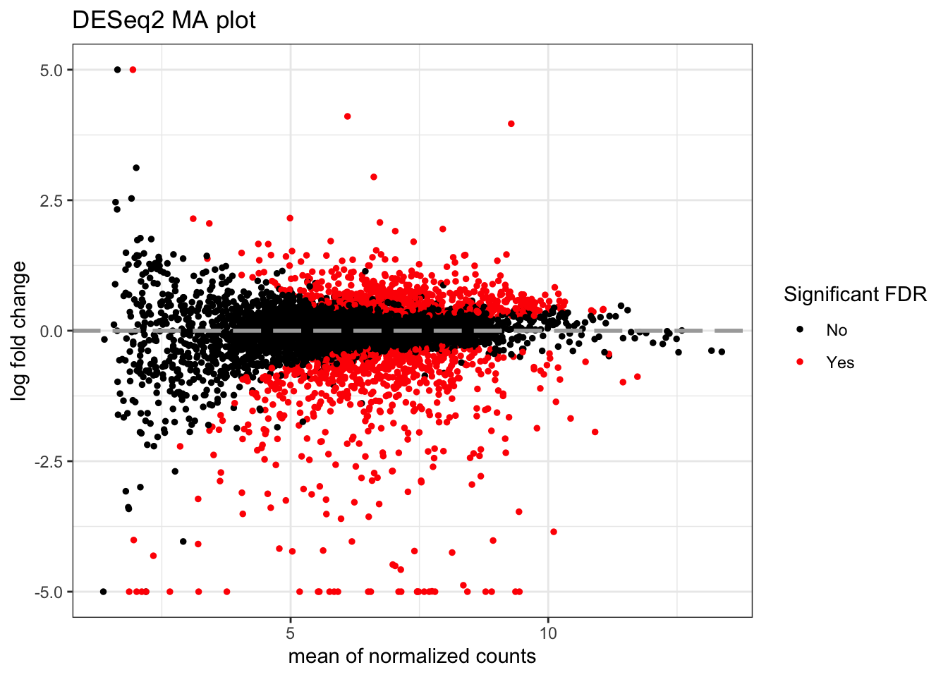
#plot MA for DESeq2 using ggplot2
topTags_DESeq2 %>%
mutate(
`Significant FDR` = case_when(padj < sig_cutoff ~ "Yes",
.default = "No"),
delabel = case_when(
padj < sig_cutoff & abs(log2FoldChange) > FC_label_cutoff ~ ORF,
.default = NA)
) %>%
ggplot(aes(log(baseMean), log2FoldChange, color = `Significant FDR`, label = delabel)) +
geom_point(size=1) +
scale_y_continuous(limits=c(-5, 5), oob=squish) +
geom_hline(yintercept = 0, colour="darkgrey", linewidth=1, linetype="longdash") +
labs(x="mean of normalized counts", y="log fold change") +
# ggrepel::geom_text_repel(size = 1.5) +
scale_color_manual(values = c("black", "red")) +
theme_bw() +
ggtitle("DESeq2 MA plot")
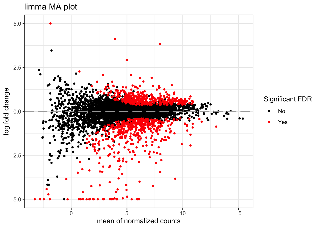
#plot MA for limma using ggplot2
topTags_limma %>%
mutate(
`Significant FDR` = case_when(adj.P.Val < sig_cutoff ~ "Yes",
.default = "No"),
delabel = case_when(
adj.P.Val < sig_cutoff & abs(logFC) > FC_label_cutoff ~ ORF,
.default = NA)
) %>%
ggplot(aes(AveExpr, logFC, color = `Significant FDR`, label = delabel)) +
geom_point(size=1) +
scale_y_continuous(limits=c(-5, 5), oob=squish) +
geom_hline(yintercept = 0, colour="darkgrey", linewidth=1, linetype="longdash") +
labs(x="mean of normalized counts", y="log fold change") +
# ggrepel::geom_text_repel(size = 1.5) +
scale_color_manual(values = c("black", "red")) +
theme_bw() +
ggtitle("limma MA plot")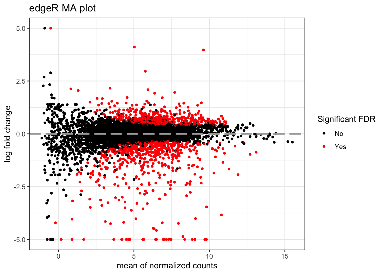
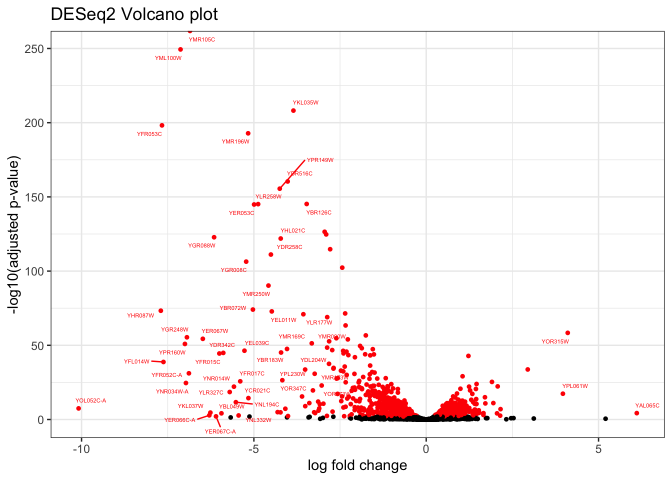
9.4 Volcano Plot
# change the dimensions of the output figure by clicking the gear icon in topright corner of the code chunk > "use custom figure size"
topTags_edgeR %>%
mutate(`Significant FDR` = case_when(
FDR < sig_cutoff ~ "Yes",
.default = "No"),
delabel = case_when(FDR < sig_cutoff & abs(logFC) > FC_label_cutoff ~ ORF,
.default = NA)) %>%
ggplot(aes(x = logFC, -log10(FDR), color = `Significant FDR`, label = delabel)) +
geom_point(size = 1) +
ggrepel::geom_text_repel(size = 1.5) +
labs(x = "log fold change", y = "-log10(adjusted p-value)") +
theme_bw() +
guides(color="none") +
scale_color_manual(values = c("black", "red")) +
ggtitle("edgeR Volcano plot")## Warning: Removed 5556 rows containing missing values (`geom_text_repel()`).topTags_DESeq2 %>%
mutate(
`Significant FDR` = case_when(padj < sig_cutoff ~ "Yes",
.default = "No"),
delabel = case_when(
padj < sig_cutoff & abs(log2FoldChange) > FC_label_cutoff ~ ORF,
.default = NA)
) %>%
ggplot(aes(log2FoldChange,-log10(padj), color = `Significant FDR`, label = delabel)) +
geom_point(size = 1) +
ggrepel::geom_text_repel(size = 1.5) +
labs(x = "log fold change", y = "-log10(adjusted p-value)") +
theme_bw() +
guides(color="none") +
scale_color_manual(values = c("black", "red")) +
ggtitle("DESeq2 Volcano plot")## Warning: Removed 5559 rows containing missing values (`geom_text_repel()`).## Warning: ggrepel: 13 unlabeled data points (too many overlaps). Consider
## increasing max.overlapstopTags_limma %>%
mutate(
`Significant FDR` = case_when(adj.P.Val < sig_cutoff ~ "Yes",
.default = "No"),
delabel = case_when(
adj.P.Val < sig_cutoff & abs(logFC) > FC_label_cutoff ~ ORF,
.default = NA)
) %>%
ggplot(aes(x=logFC, y=-log10(P.Value), color = `Significant FDR`, label = delabel)) +
geom_point(size = 1) +
ggrepel::geom_text_repel(size = 1.5) +
labs(x = "log fold change", y = "-log10(UNADJUSTED p-value)") +
theme_bw() +
guides(color="none") +
scale_color_manual(values = c("black", "red")) +
ggtitle("limma Volcano plot")## Warning: Removed 5557 rows containing missing values (`geom_text_repel()`).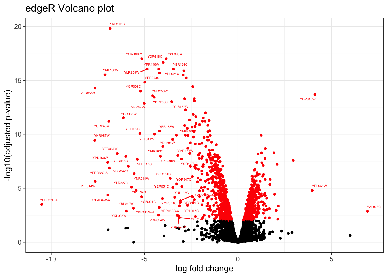

9.5 Using Glimma for an interactive visualization
9.5.1 MA plots
# load in res objects for both limma and edgeR
res_limma <- readRDS("~/Desktop/Genomic_Data_Analysis/Analysis/limma/yeast_res_limma.Rds")
res_edgeR <- readRDS("~/Desktop/Genomic_Data_Analysis/Analysis/edgeR/yeast_res_edgeR.Rds")
# code to pull it from github:
# res_limma <- read_rds("https://github.com/clstacy/GenomicDataAnalysis_Fa23/raw/main/analysis/yeast_res_limma.Rds")
# res_edgeR <- read_rds("https://github.com/clstacy/GenomicDataAnalysis_Fa23/raw/main/analysis/yeast_res_edgeR.Rds")
# load in the DGE lists for each
y_limma <- readRDS("~/Desktop/Genomic_Data_Analysis/Analysis/limma/yeast_y_limma.Rds")
y_edgeR <- readRDS("~/Desktop/Genomic_Data_Analysis/Analysis/edgeR/yeast_y_edgeR.Rds")
# again, alternative code to pull from github
# y_limma <- read_rds("https://github.com/clstacy/GenomicDataAnalysis_Fa23/raw/main/analysis/yeast_y_limma.Rds")
# y_edgeR <- read_rds("https://github.com/clstacy/GenomicDataAnalysis_Fa23/raw/main/analysis/yeast_y_edgeR.Rds")
glimmaMA(res_limma, dge = y_limma)## Warning in buildXYData(table, status, main, display.columns, anno, counts, :
## count transform requested but not all count values are integers.9.6 Generating bar graph summaries
This visualization approach compresses relevant information, so it’s generally a discouraged approach for visualizing DE data. However, it is done, so if it is useful for your study, here is how you could do it.
# let's use the res_all object from the 08_DE_limma exercise:
res_all_limma <- read_rds('https://github.com/clstacy/GenomicDataAnalysis_Fa23/raw/main/analysis/yeast_res_allContrasts_limma.Rds')
decideTests_all_edgeR <-
read.delim(
'https://github.com/clstacy/GenomicDataAnalysis_Fa23/raw/main/analysis/yeast_decideTests_allContrasts_edgeR.tsv',
sep = "\t",
header = T,
row.names = 1
) %>% rownames_to_column("gene")
res_all_limma %>%
decideTests(p.value = 0.05, lfc = 0) %>%
as.data.frame() %>%
rownames_to_column("gene") %>%
pivot_longer(c(-gene), names_to = "contrast", values_to = "DE_direction") %>%
group_by(contrast) %>%
summarise(
upregulated = sum(DE_direction == 1),
downregulated = sum(DE_direction == -1)
) %>%
pivot_longer(c(-contrast), names_to = "DE_direction", values_to = "n_genes") %>%
ggplot(aes(x = contrast, y = n_genes, fill = DE_direction)) +
geom_col(position = "dodge") +
theme_bw() +
coord_flip() +
geom_text(aes(label = n_genes),
position = position_dodge(width = .9),
hjust = "inward") +
labs(y="Number of DE genes") +
ggtitle("Summary of DE genes by contrast (limma)")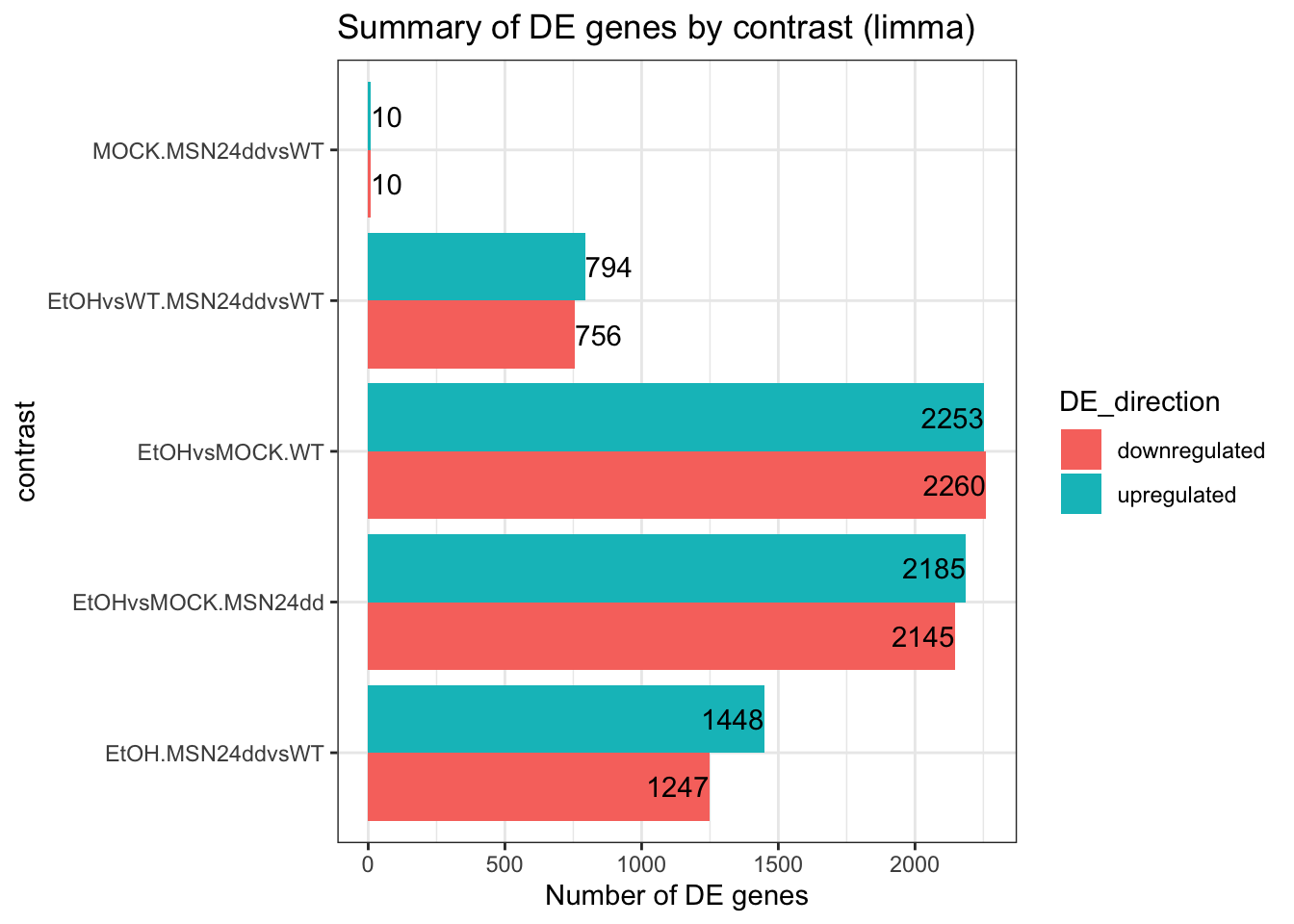
# how to do the same for edgeR
decideTests_all_edgeR %>%
pivot_longer(c(-gene), names_to = "contrast", values_to = "DE_direction") %>%
group_by(contrast) %>%
summarise(
upregulated = sum(DE_direction == 1),
downregulated = sum(DE_direction == -1)
) %>%
pivot_longer(-contrast, names_to = "DE_direction", values_to = "n_genes") %>%
mutate(contrast = fct_reorder(contrast, 1/(1+n_genes))) %>%
ggplot(aes(x = contrast, y = n_genes, fill = DE_direction)) +
geom_col(position = "dodge") +
theme_bw() +
coord_flip() +
scale_x_discrete(labels = function(x) str_wrap(x, width = 10)) +
geom_text(aes(label = n_genes),
position = position_dodge(width = .9),
hjust = "inward") +
labs(y="Number of DE genes") +
ggtitle("Summary of DE genes by contrast (edgeR)")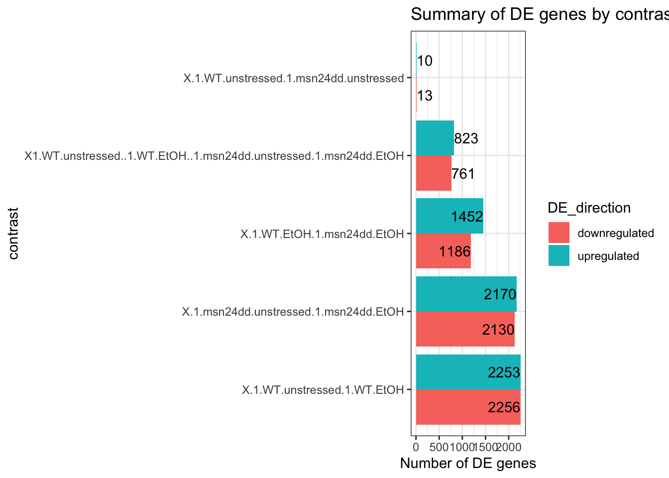
If we want to show the same amount of information, in a more informative way, a venn diagram is often a better alternative. Here’s an easy way to get that visualization if you use either edgeR or limma for your analysis.
# same as before, we can make the plot from the decideTests output
res_all_limma %>%
decideTests(p.value = 0.01, lfc = 0) %>%
vennDiagram(include=c("up", "down"),
lwd=0.75,
mar=rep(2,4), # increase margin size
counts.col= c("red", "blue"),
show.include=TRUE)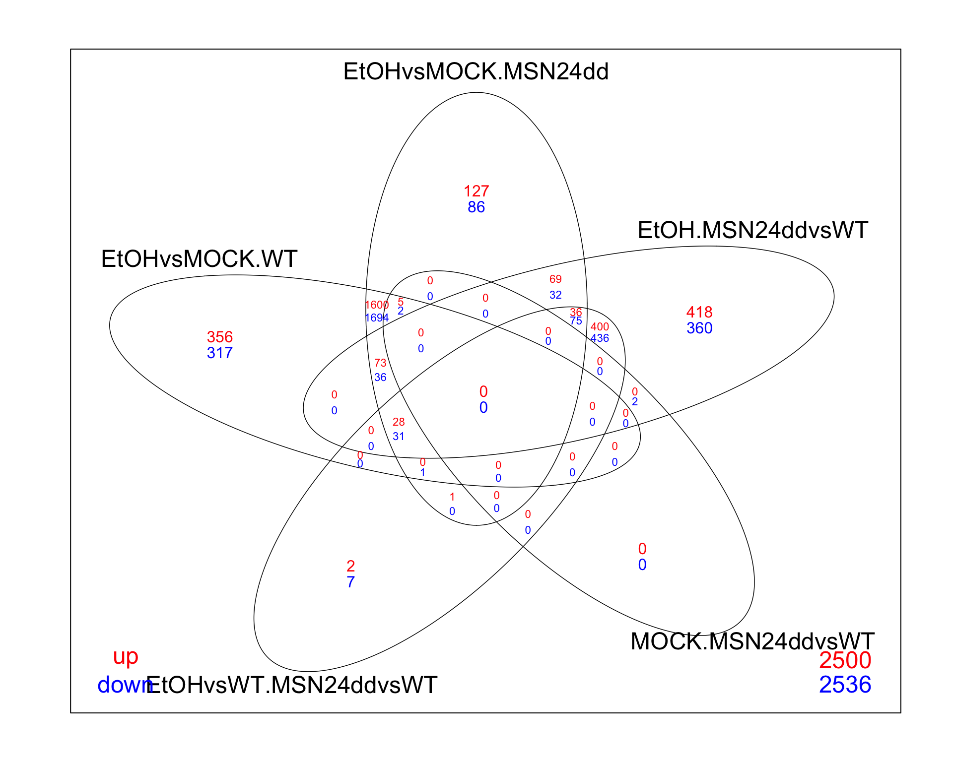
decideTests_all_edgeR %>%
column_to_rownames("gene") %>%
vennDiagram(include=c("up", "down"),
lwd=0.75,
mar=rep(4,4), # increase margin size
counts.col= c("red", "blue"),
show.include=TRUE)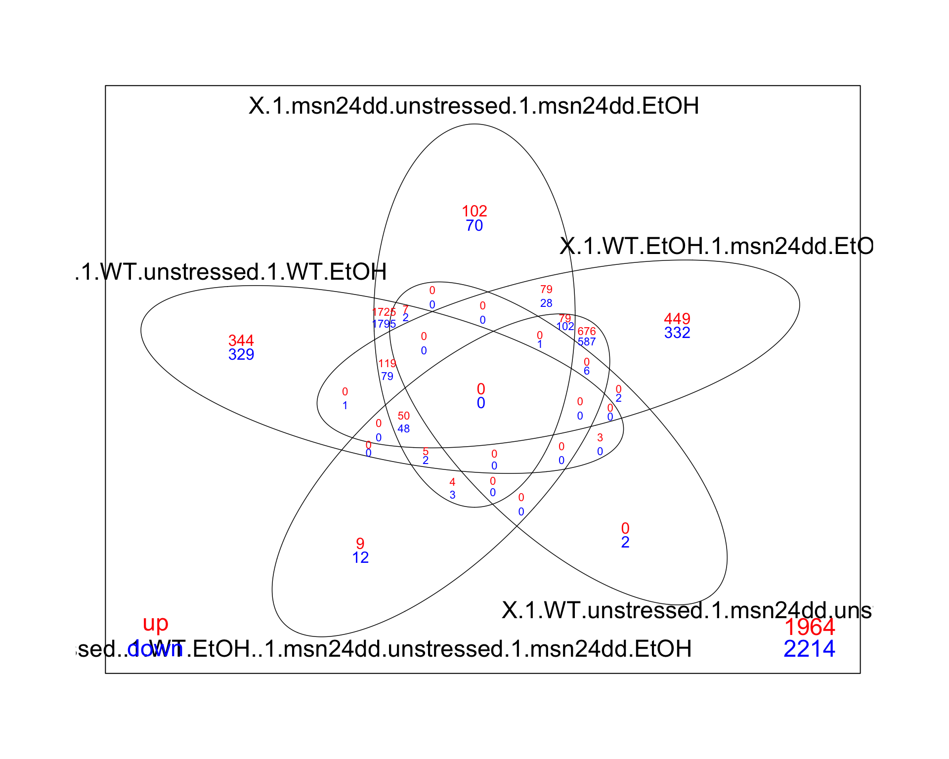
Venn diagrams are useful for showing gene counts as well as there overlaps between contrasts. A useful gui based web-page for creating venn diagrams inclues: https://eulerr.co/. If you enjoy coding, it also exists as an R package (https://cran.r-project.org/web/packages/eulerr/index.html).
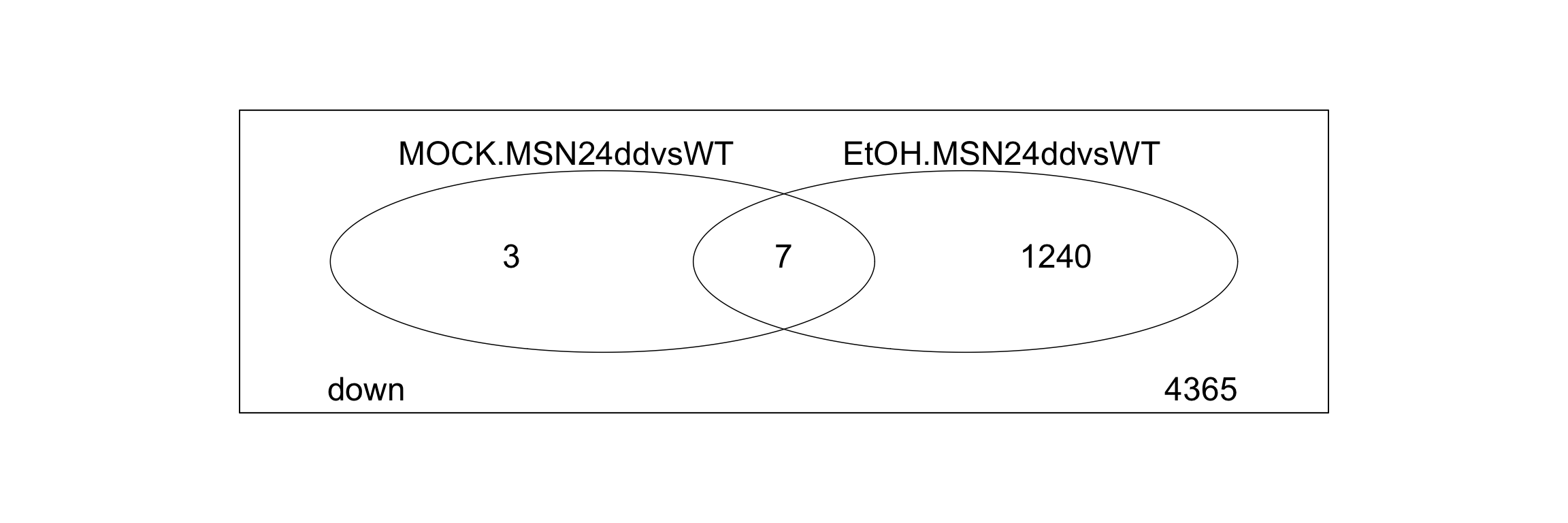
9.7 Exercise
- Modify the code below to find out how many genes are upregulated (p.value < 0.01 and |lfc| > 1) in the ethanol stress response of both WT cells and msn2/4 mutants.
## [1] "EtOHvsMOCK.WT" "EtOHvsMOCK.MSN24dd" "EtOH.MSN24ddvsWT"
## [4] "MOCK.MSN24ddvsWT" "EtOHvsWT.MSN24ddvsWT"# select the correct two and replace them below
res_all_limma %>%
decideTests(p.value = 0.05, lfc = 0) %>%
data.frame() %>%
# change the columns selected in this select command
dplyr::select(c("MOCK.MSN24ddvsWT", "EtOH.MSN24ddvsWT")) %>%
vennDiagram(include="down",
lwd=0.75,
mar=rep(0,4), # increase margin size
# counts.col= c("red", "blue"),
show.include=TRUE
)
R version 4.3.1 (2023-06-16)
Platform: aarch64-apple-darwin20 (64-bit)
locale: en_US.UTF-8||en_US.UTF-8||en_US.UTF-8||C||en_US.UTF-8||en_US.UTF-8
attached base packages: stats4, stats, graphics, grDevices, utils, datasets, methods and base
other attached packages: ggrepel(v.0.9.4), viridis(v.0.6.4), viridisLite(v.0.4.2), scales(v.1.2.1), Glimma(v.2.10.0), DESeq2(v.1.40.2), edgeR(v.3.42.4), limma(v.3.56.2), reactable(v.0.4.4), webshot2(v.0.1.1), statmod(v.1.5.0), Rsubread(v.2.14.2), ShortRead(v.1.58.0), GenomicAlignments(v.1.36.0), SummarizedExperiment(v.1.30.2), MatrixGenerics(v.1.12.3), matrixStats(v.1.0.0), Rsamtools(v.2.16.0), GenomicRanges(v.1.52.1), Biostrings(v.2.68.1), GenomeInfoDb(v.1.36.4), XVector(v.0.40.0), BiocParallel(v.1.34.2), Rfastp(v.1.10.0), org.Sc.sgd.db(v.3.17.0), AnnotationDbi(v.1.62.2), IRanges(v.2.34.1), S4Vectors(v.0.38.2), Biobase(v.2.60.0), BiocGenerics(v.0.46.0), clusterProfiler(v.4.8.2), ggVennDiagram(v.1.2.3), tidytree(v.0.4.5), igraph(v.1.5.1), janitor(v.2.2.0), BiocManager(v.1.30.22), pander(v.0.6.5), knitr(v.1.44), here(v.1.0.1), lubridate(v.1.9.3), forcats(v.1.0.0), stringr(v.1.5.0), dplyr(v.1.1.3), purrr(v.1.0.2), readr(v.2.1.4), tidyr(v.1.3.0), tibble(v.3.2.1), ggplot2(v.3.4.4), tidyverse(v.2.0.0) and pacman(v.0.5.1)
loaded via a namespace (and not attached): splines(v.4.3.1), later(v.1.3.1), bitops(v.1.0-7), ggplotify(v.0.1.2), polyclip(v.1.10-6), lifecycle(v.1.0.3), rprojroot(v.2.0.3), processx(v.3.8.2), lattice(v.0.21-9), MASS(v.7.3-60), magrittr(v.2.0.3), sass(v.0.4.7), rmarkdown(v.2.25), jquerylib(v.0.1.4), yaml(v.2.3.7), cowplot(v.1.1.1), chromote(v.0.1.2), DBI(v.1.1.3), RColorBrewer(v.1.1-3), abind(v.1.4-5), zlibbioc(v.1.46.0), ggraph(v.2.1.0), RCurl(v.1.98-1.12), yulab.utils(v.0.1.0), tweenr(v.2.0.2), GenomeInfoDbData(v.1.2.10), enrichplot(v.1.20.0), codetools(v.0.2-19), DelayedArray(v.0.26.7), DOSE(v.3.26.1), ggforce(v.0.4.1), tidyselect(v.1.2.0), aplot(v.0.2.2), farver(v.2.1.1), jsonlite(v.1.8.7), tidygraph(v.1.2.3), tools(v.4.3.1), treeio(v.1.24.3), Rcpp(v.1.0.11), glue(v.1.6.2), gridExtra(v.2.3), xfun(v.0.40), qvalue(v.2.32.0), websocket(v.1.4.1), withr(v.2.5.1), fastmap(v.1.1.1), latticeExtra(v.0.6-30), fansi(v.1.0.5), digest(v.0.6.33), timechange(v.0.2.0), R6(v.2.5.1), gridGraphics(v.0.5-1), colorspace(v.2.1-0), GO.db(v.3.17.0), jpeg(v.0.1-10), RSQLite(v.2.3.1), utf8(v.1.2.3), generics(v.0.1.3), data.table(v.1.14.8), graphlayouts(v.1.0.1), httr(v.1.4.7), htmlwidgets(v.1.6.2), S4Arrays(v.1.0.6), scatterpie(v.0.2.1), pkgconfig(v.2.0.3), gtable(v.0.3.4), blob(v.1.2.4), hwriter(v.1.3.2.1), shadowtext(v.0.1.2), htmltools(v.0.5.6.1), bookdown(v.0.36), fgsea(v.1.26.0), png(v.0.1-8), snakecase(v.0.11.1), ggfun(v.0.1.3), rstudioapi(v.0.15.0), tzdb(v.0.4.0), reshape2(v.1.4.4), rjson(v.0.2.21), nlme(v.3.1-163), cachem(v.1.0.8), RVenn(v.1.1.0), parallel(v.4.3.1), HDO.db(v.0.99.1), pillar(v.1.9.0), grid(v.4.3.1), vctrs(v.0.6.4), promises(v.1.2.1), evaluate(v.0.22), cli(v.3.6.1), locfit(v.1.5-9.8), compiler(v.4.3.1), rlang(v.1.1.1), crayon(v.1.5.2), labeling(v.0.4.3), interp(v.1.1-4), ps(v.1.7.5), plyr(v.1.8.9), fs(v.1.6.3), stringi(v.1.7.12), deldir(v.1.0-9), munsell(v.0.5.0), lazyeval(v.0.2.2), GOSemSim(v.2.26.1), Matrix(v.1.6-1.1), hms(v.1.1.3), patchwork(v.1.1.3), bit64(v.4.0.5), KEGGREST(v.1.40.1), memoise(v.2.0.1), bslib(v.0.5.1), ggtree(v.3.8.2), fastmatch(v.1.1-4), bit(v.4.0.5), downloader(v.0.4), ape(v.5.7-1) and gson(v.0.1.0)