Chapter 6 Differential Expression: EdgeR
last updated: 2023-10-27
Package Install
As usual, make sure we have the right packages for this exercise
if (!require("pacman")) install.packages("pacman"); library(pacman)

# let's load all of the files we were using and want to have again today
p_load("tidyverse", "knitr", "readr",
       "pander", "BiocManager",
       "dplyr", "stringr",
       "statmod", # required dependency, need to load manually on some macOS versions.
       "purrr", # for working with lists (beautify column names)
       "webshot2", # allow for pdf of output table.
       "reactable") # for pretty tables.

# We also need these Bioconductor packages today.
p_load("edgeR", "AnnotationDbi", "org.Sc.sgd.db")
6.1 Description
This will be our first differential expression analysis workflow, converting gene counts across samples into meaningful information about genes that appear to be significantly differentially expressed between samples
6.2 Learning outcomes
At the end of this exercise, you should be able to:
- Generate a table of sample metadata.
- Filter low counts and normalize count data.
- Utilize the edgeR package to identify differentially expressed genes.
6.3 Loading in the featureCounts object
We saved this file in the last exercise (05_Read_Counting.Rmd) from the
RSubread package. Now we can load that object back in and assign it to
the variable fc. Be sure to change the file path if you have saved it
in a different location.
path_fc_object <- path.expand("~/Desktop/Genomic_Data_Analysis/Data/Counts/Rsubread/rsubread.yeast_fc_output.Rds")

counts_subset <- readRDS(file = path_fc_object)$counts
We generated those counts on a subset of the fastq files, but we can load the complete count file with the command below. This file has been generated with the full size fastq files with Salmon.
counts <-
  read.delim(
    'https://github.com/clstacy/GenomicDataAnalysis_Fa23/raw/main/data/ethanol_stress/counts/salmon.gene_counts.merged.nonsubsamp.tsv',
    sep = "\t",
    header = T,
    row.names = 1
  )
So far, we’ve been able to process all of the fastq files without much information about what each sample is in the experimental design. Now, we need the metadata for the samples. Note that the order matters for these files
To find the order of files we need, we can get just the part of the column name before the first “.” symbol with this command:
## YPS606_MSN24_ETOH_REP1_R1 YPS606_MSN24_ETOH_REP2_R1 YPS606_MSN24_ETOH_REP3_R1 YPS606_MSN24_ETOH_REP4_R1 YPS606_MSN24_MOCK_REP1_R1 YPS606_MSN24_MOCK_REP2_R1 YPS606_MSN24_MOCK_REP3_R1 YPS606_MSN24_MOCK_REP4_R1 YPS606_WT_ETOH_REP1_R1 YPS606_WT_ETOH_REP2_R1 YPS606_WT_ETOH_REP3_R1 YPS606_WT_ETOH_REP4_R1 YPS606_WT_MOCK_REP1_R1 YPS606_WT_MOCK_REP2_R1 YPS606_WT_MOCK_REP3_R1 YPS606_WT_MOCK_REP4_R1sample_metadata <- tribble(
~Sample, ~Genotype, ~Condition,
"YPS606_MSN24_ETOH_REP1_R1", "msn24dd", "EtOH",
"YPS606_MSN24_ETOH_REP2_R1", "msn24dd", "EtOH",
"YPS606_MSN24_ETOH_REP3_R1", "msn24dd", "EtOH",
"YPS606_MSN24_ETOH_REP4_R1", "msn24dd", "EtOH",
"YPS606_MSN24_MOCK_REP1_R1", "msn24dd", "unstressed",
"YPS606_MSN24_MOCK_REP2_R1", "msn24dd", "unstressed",
"YPS606_MSN24_MOCK_REP3_R1", "msn24dd", "unstressed",
"YPS606_MSN24_MOCK_REP4_R1", "msn24dd", "unstressed",
"YPS606_WT_ETOH_REP1_R1", "WT", "EtOH",
"YPS606_WT_ETOH_REP2_R1", "WT", "EtOH",
"YPS606_WT_ETOH_REP3_R1", "WT", "EtOH",
"YPS606_WT_ETOH_REP4_R1", "WT", "EtOH",
"YPS606_WT_MOCK_REP1_R1", "WT", "unstressed",
"YPS606_WT_MOCK_REP2_R1", "WT", "unstressed",
"YPS606_WT_MOCK_REP3_R1", "WT", "unstressed",
"YPS606_WT_MOCK_REP4_R1", "WT", "unstressed") |>
# Create a new column that combines the Genotype and Condition value
mutate(Group = factor(
paste(Genotype, Condition, sep = "."),
levels = c(
"WT.unstressed","WT.EtOH",
"msn24dd.unstressed", "msn24dd.EtOH"
)
)) |>
# make Condition and Genotype a factor (with baseline as first level) for edgeR
mutate(
Genotype = factor(Genotype,
levels = c("WT", "msn24dd")),
Condition = factor(Condition,
levels = c("unstressed", "EtOH"))
)Now, let’s create a design matrix with this information
##    groupWT.unstressed groupWT.EtOH groupmsn24dd.unstressed groupmsn24dd.EtOH
## 1                   0            0                       0                 1
## 2                   0            0                       0                 1
## 3                   0            0                       0                 1
## 4                   0            0                       0                 1
## 5                   0            0                       1                 0
## 6                   0            0                       1                 0
## 7                   0            0                       1                 0
## 8                   0            0                       1                 0
## 9                   0            1                       0                 0
## 10                  0            1                       0                 0
## 11                  0            1                       0                 0
## 12                  0            1                       0                 0
## 13                  1            0                       0                 0
## 14                  1            0                       0                 0
## 15                  1            0                       0                 0
## 16                  1            0                       0                 0
## attr(,"assign")
## [1] 1 1 1 1
## attr(,"contrasts")
## attr(,"contrasts")$group
## [1] "contr.treatment"## WT.unstressed WT.EtOH msn24dd.unstressed msn24dd.EtOH
## 1 0 0 0 1
## 2 0 0 0 1
## 3 0 0 0 1
## 4 0 0 0 1
## 5 0 0 1 0
## 6 0 0 1 0
## 7 0 0 1 0
## 8 0 0 1 0
## 9 0 1 0 0
## 10 0 1 0 0
## 11 0 1 0 0
## 12 0 1 0 0
## 13 1 0 0 0
## 14 1 0 0 0
## 15 1 0 0 0
## 16 1 0 0 0
## attr(,"assign")
## [1] 1 1 1 1
## attr(,"contrasts")
## attr(,"contrasts")$group
## [1] "contr.treatment"6.4 Count loading and Annotation
The count matrix is used to construct a DGEList class object. This is the main data class in the edgeR package. The DGEList object is used to store all the information required to fit a generalized linear model to the data, including library sizes and dispersion estimates as well as counts for each gene.
##                                        group lib.size norm.factors
## YPS606_MSN24_ETOH_REP1_R1       msn24dd.EtOH 17409481            1
## YPS606_MSN24_ETOH_REP2_R1       msn24dd.EtOH 14055425            1
## YPS606_MSN24_ETOH_REP3_R1       msn24dd.EtOH 13127876            1
## YPS606_MSN24_ETOH_REP4_R1       msn24dd.EtOH 16655559            1
## YPS606_MSN24_MOCK_REP1_R1 msn24dd.unstressed 12266723            1
## YPS606_MSN24_MOCK_REP2_R1 msn24dd.unstressed 11781244            1
## YPS606_MSN24_MOCK_REP3_R1 msn24dd.unstressed 11340274            1
## YPS606_MSN24_MOCK_REP4_R1 msn24dd.unstressed 13024330            1
## YPS606_WT_ETOH_REP1_R1               WT.EtOH 15422048            1
## YPS606_WT_ETOH_REP2_R1               WT.EtOH 14924728            1
## YPS606_WT_ETOH_REP3_R1               WT.EtOH 14738753            1
## YPS606_WT_ETOH_REP4_R1               WT.EtOH 12203133            1
## YPS606_WT_MOCK_REP1_R1         WT.unstressed 13592206            1
## YPS606_WT_MOCK_REP2_R1         WT.unstressed 12921965            1
## YPS606_WT_MOCK_REP3_R1         WT.unstressed 13128396            1
## YPS606_WT_MOCK_REP4_R1         WT.unstressed 15568155            1
Human-readable gene symbols can also be added to complement the gene ID for each gene, using the annotation in the org.Sc.sgd.db package.
## 'select()' returned 1:1 mapping between keys and columns## ORF SGD GENENAME
## 1 YIL170W S000001432 HXT12
## 2 YIL175W S000001437 <NA>
## 3 YPL276W S000006197 <NA>
## 4 YFL056C S000001838 AAD6
## 5 YCL074W S000000579 <NA>
## 6 YAR061W S000000087 <NA>6.5 Filtering to remove low counts
Genes with very low counts across all libraries provide little evidence for differential expression. In addition, the pronounced discreteness of these counts interferes with some of the statistical approximations that are used later in the pipeline. These genes should be filtered out prior to further analysis. Here, we will retain a gene only if it is expressed at a count-per-million (CPM) above 0.7 in at least four samples.
##    Mode   FALSE    TRUE
## logical     956    5615
Where did those cutoff numbers come from?
As a general rule, we don’t want to exclude a gene that is expressed in only one group, so a cutoff number equal to the number of replicates can be a good starting point. For counts, a good threshold can be chosen by identifying the CPM that corresponds to a count of 10, which in this case would be about 0.7:
##           [,1]
## [1,] 0.7202007
Smaller CPM thresholds are usually appropriate for larger libraries.
6.6 Normalization for composition bias
TMM normalization is performed to eliminate composition biases between libraries. This generates a set of normalization factors, where the product of these factors and the library sizes defines the effective library size. The calcNormFactors function returns the DGEList argument with only the norm.factors changed.
## group lib.size norm.factors
## YPS606_MSN24_ETOH_REP1_R1 msn24dd.EtOH 17409481 1.2390418
## YPS606_MSN24_ETOH_REP2_R1 msn24dd.EtOH 14055425 1.1021628
## YPS606_MSN24_ETOH_REP3_R1 msn24dd.EtOH 13127876 1.1079633
## YPS606_MSN24_ETOH_REP4_R1 msn24dd.EtOH 16655559 1.0073996
## YPS606_MSN24_MOCK_REP1_R1 msn24dd.unstressed 12266723 1.0383288
## YPS606_MSN24_MOCK_REP2_R1 msn24dd.unstressed 11781244 1.0031950
## YPS606_MSN24_MOCK_REP3_R1 msn24dd.unstressed 11340274 0.9600073
## YPS606_MSN24_MOCK_REP4_R1 msn24dd.unstressed 13024330 0.9842621
## YPS606_WT_ETOH_REP1_R1 WT.EtOH 15422048 0.8394351
## YPS606_WT_ETOH_REP2_R1 WT.EtOH 14924728 0.9409802
## YPS606_WT_ETOH_REP3_R1 WT.EtOH 14738753 0.9881819
## YPS606_WT_ETOH_REP4_R1 WT.EtOH 12203133 0.9708557
## YPS606_WT_MOCK_REP1_R1 WT.unstressed 13592206 0.9900546
## YPS606_WT_MOCK_REP2_R1 WT.unstressed 12921965 1.0381161
## YPS606_WT_MOCK_REP3_R1 WT.unstressed 13128396 0.9002706
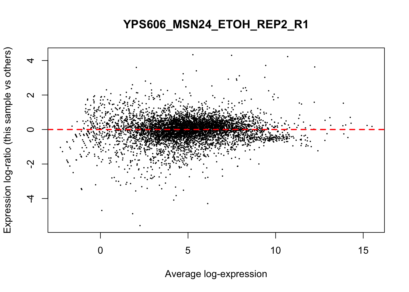
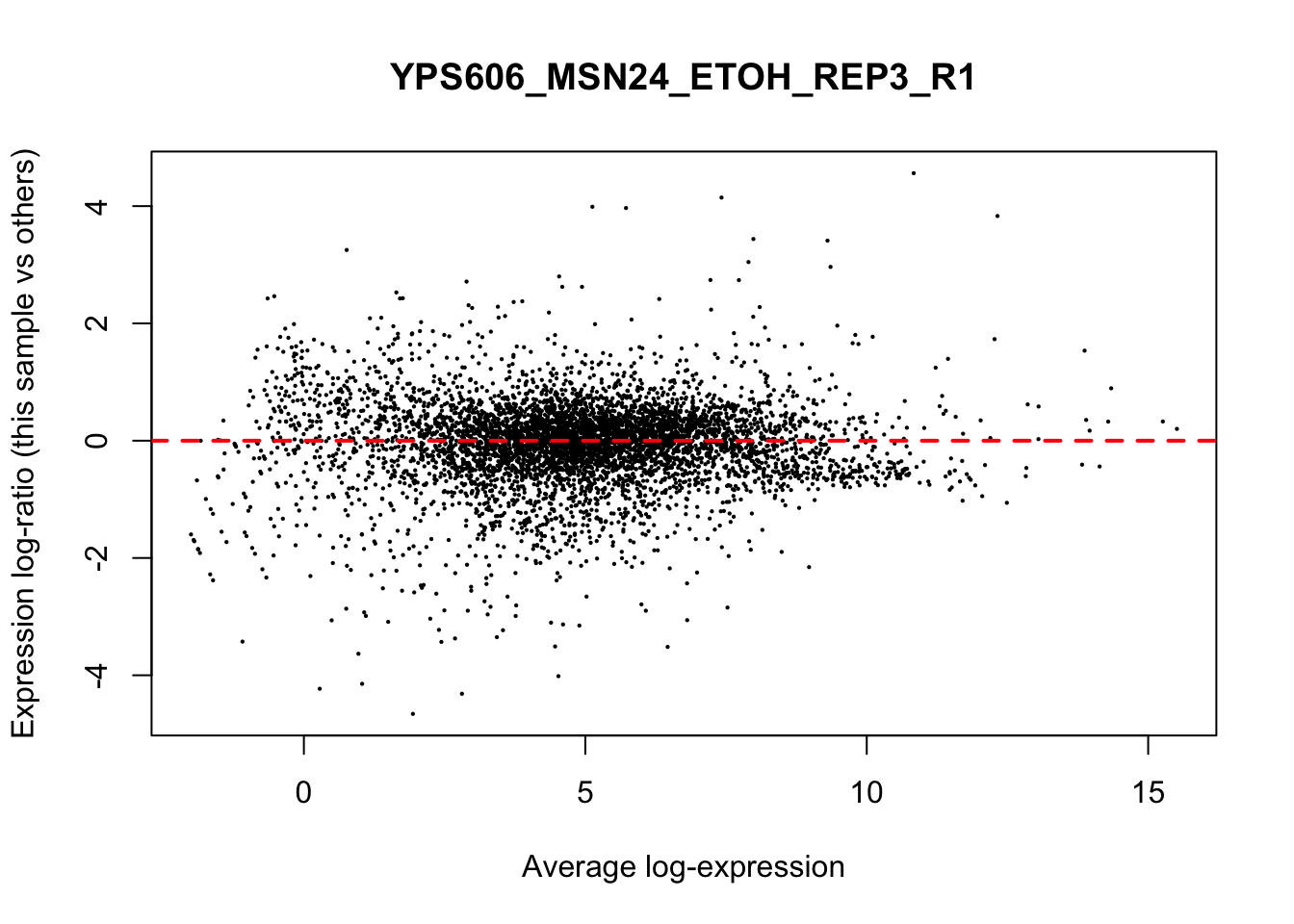
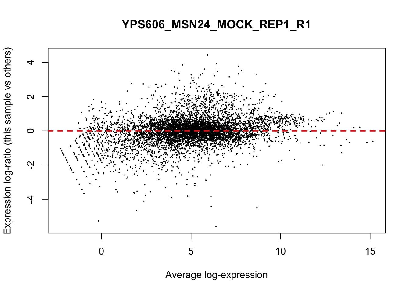
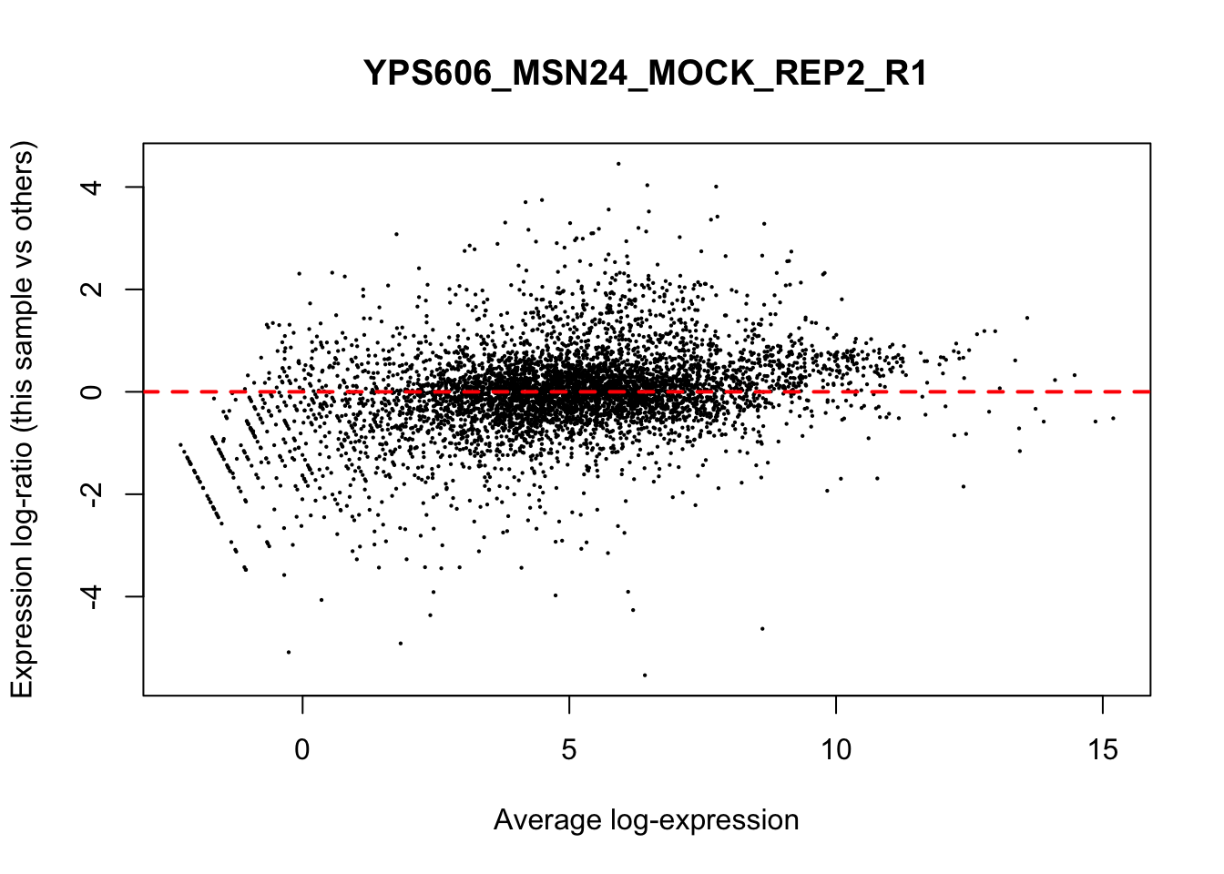
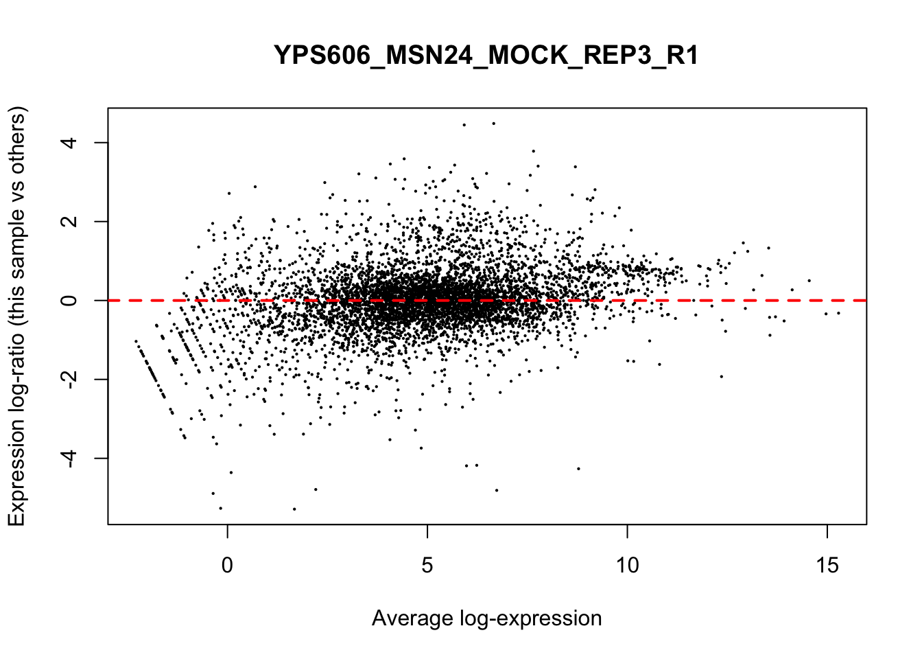
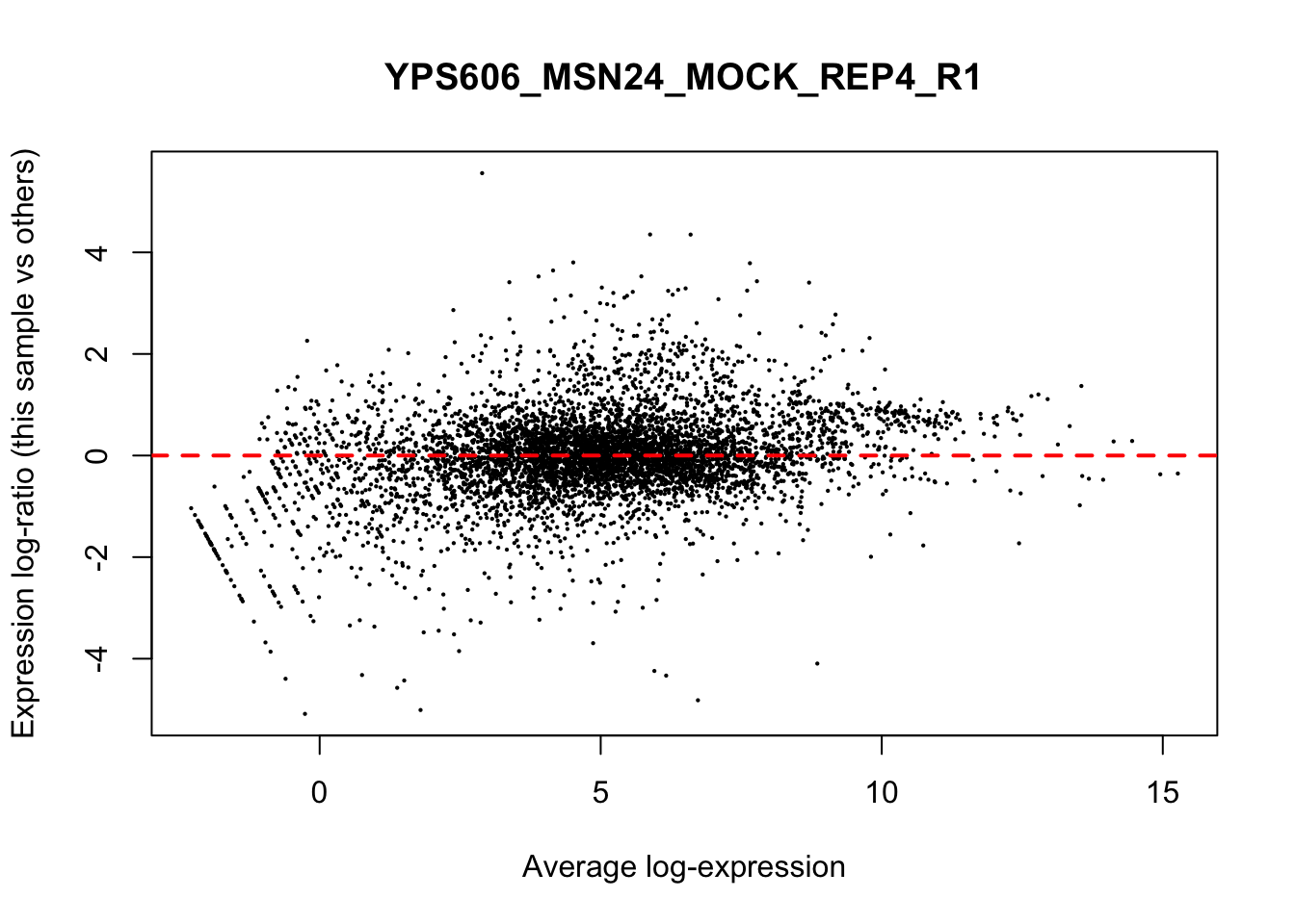
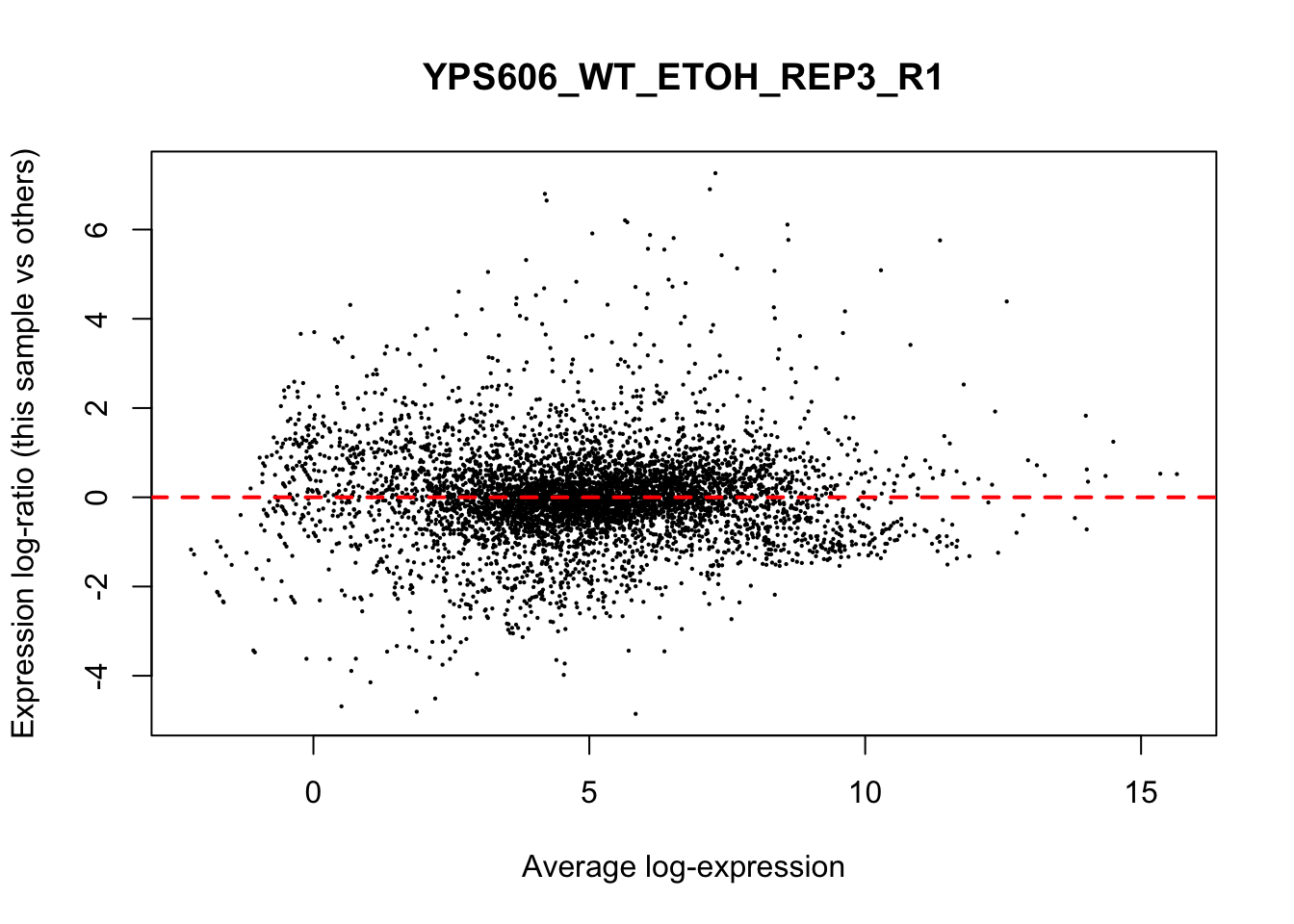
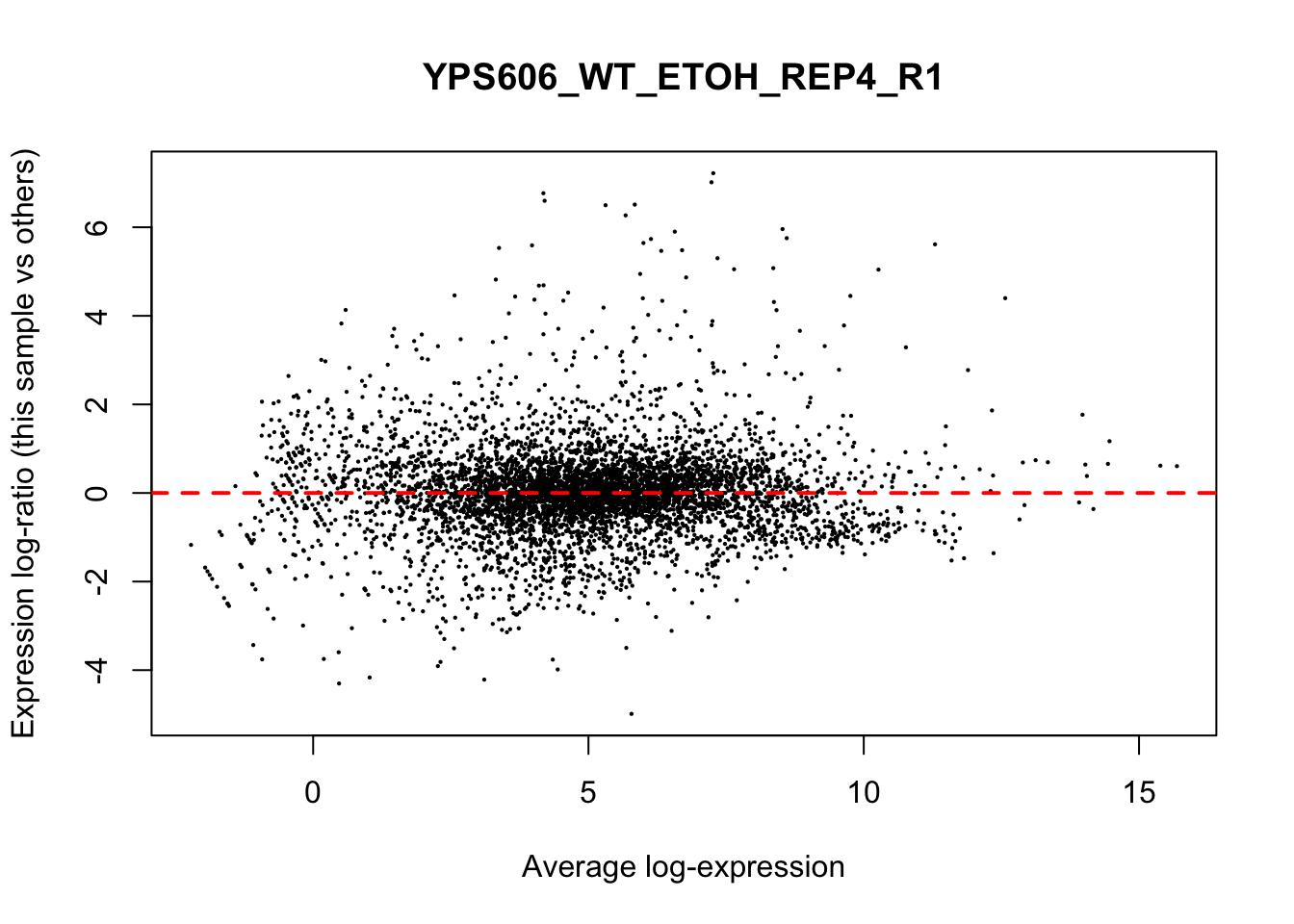
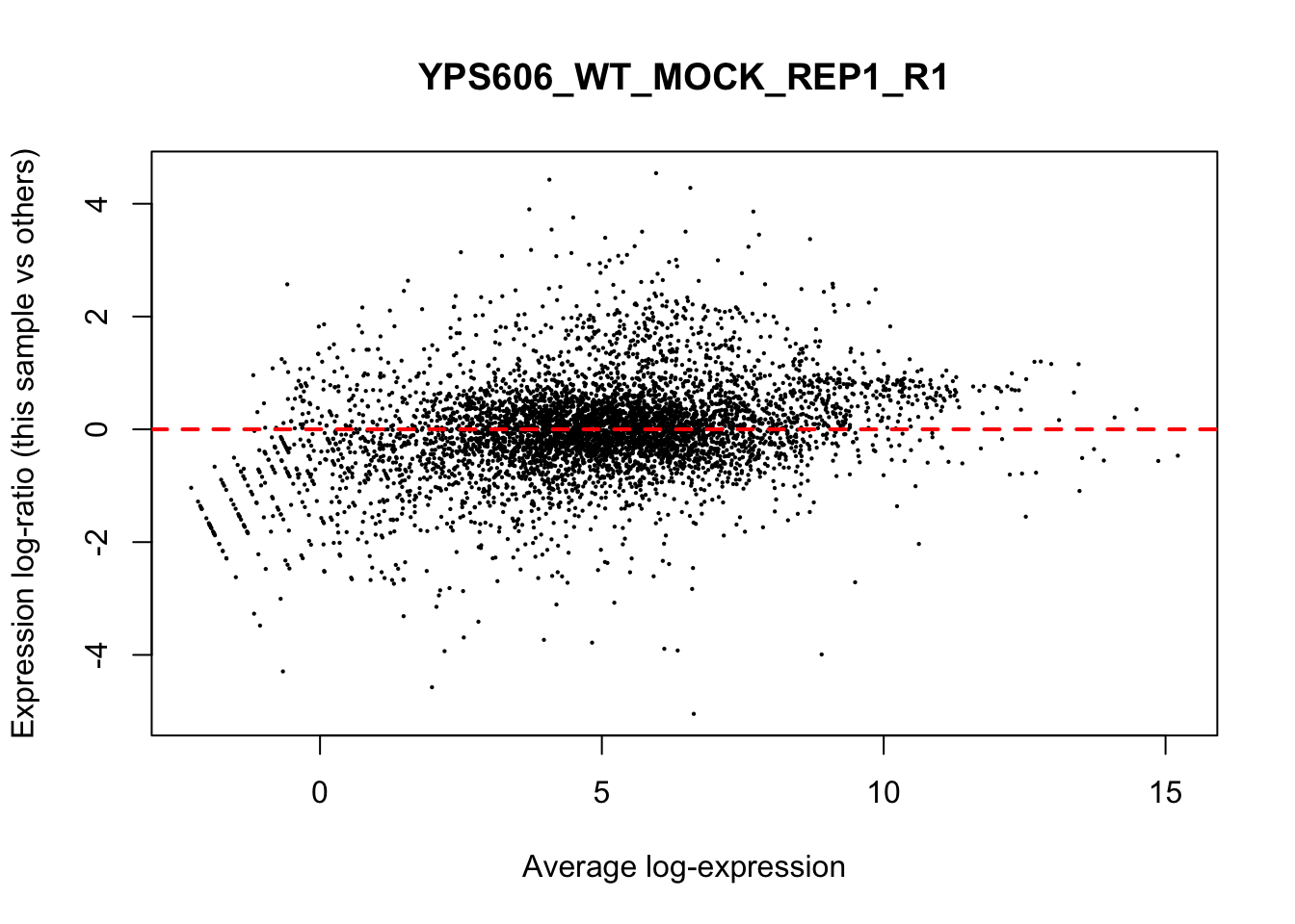
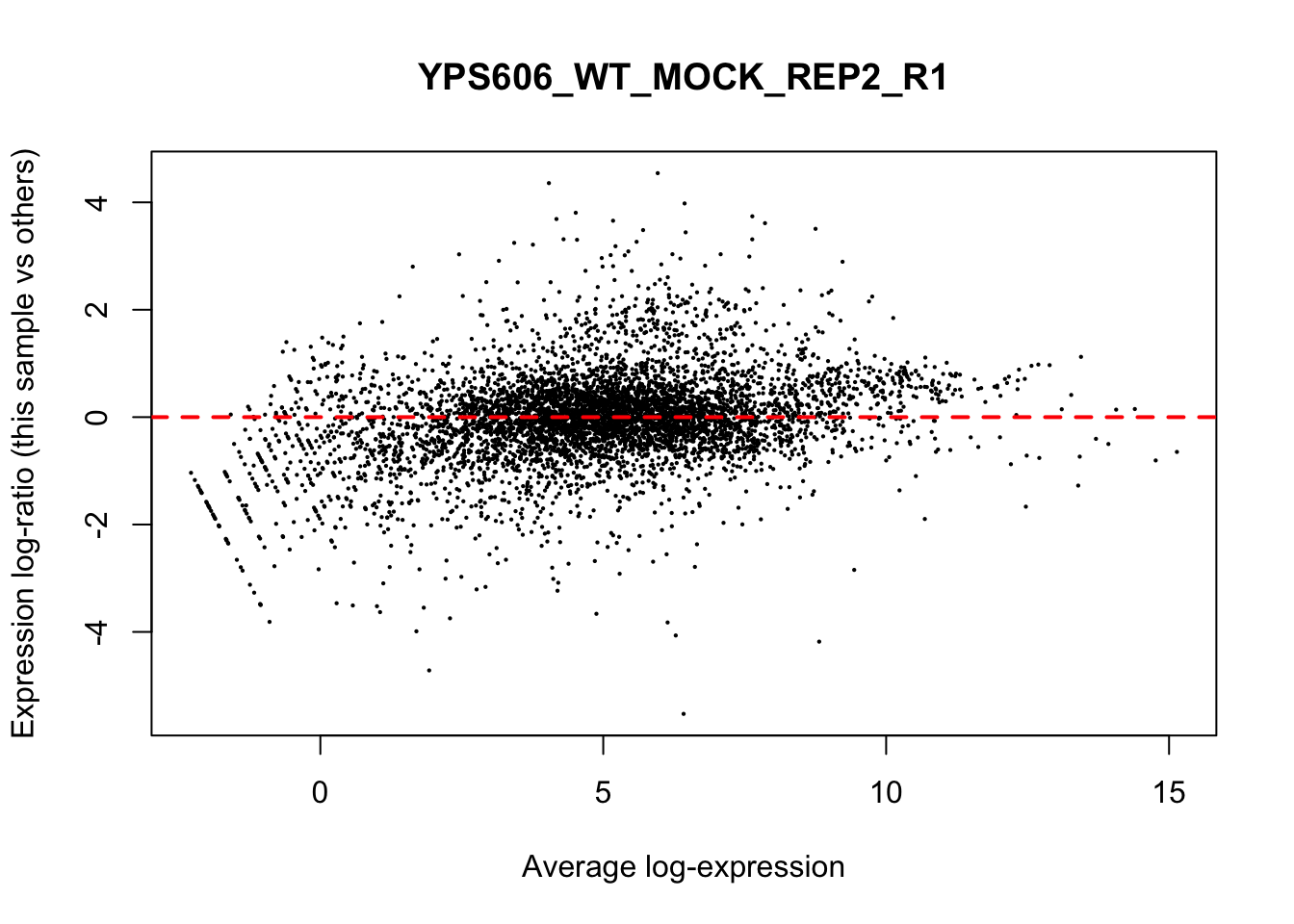
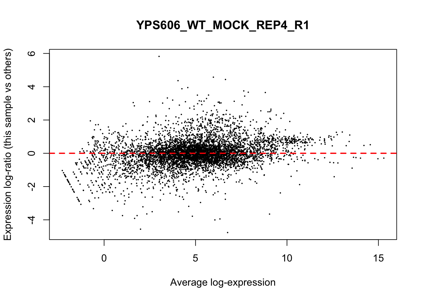
## YPS606_WT_MOCK_REP4_R1 WT.unstressed 15568155 0.9506010The normalization factors multiply to unity across all libraries. A normalization factor below unity indicates that the library size will be scaled down, as there is more suppression (i.e., composition bias) in that library relative to the other libraries. This is also equivalent to scaling the counts upwards in that sample. Conversely, a factor above unity scales up the library size and is equivalent to downscaling the counts. The performance of the TMM normalization procedure can be examined using mean- difference (MD) plots. This visualizes the library size-adjusted log-fold change between two libraries (the difference) against the average log-expression across those libraries (the mean). The below command plots an MD plot, comparing sample 1 against an artificial library constructed from the average of all other samples.
6.7 MDS plots
for (sample in 1:nrow(y$samples)) {
  plotMD(cpm(y, log=TRUE), column=sample)
  abline(h=0, col="red", lty=2, lwd=2)
}


6.8 Exploring differences between libraries
The data can be explored by generating multi-dimensional scaling (MDS) plots. This visualizes the differences between the expression profiles of different samples in two dimensions. The next plot shows the MDS plot for the yeast heatshock data.
points <- c(1,1,2,2)
colors <- rep(c("black", "red"),8)
plotMDS(y, col=colors[group], pch=points[group])
legend("topright", legend=levels(group),
     pch=points, col=colors, ncol=2)
title(main="PCA plot")
6.9 Estimate Dispersion
The trended NB dispersion is estimated using the estimateDisp function. This returns the DGEList object with additional entries for the estimated NB dispersions for all genes. These estimates can be visualized with plotBCV, which shows the root-estimate, i.e., the biological coefficient of variation for each gene
y <- estimateDisp(y, design, robust=TRUE)
plotBCV(y)
title(main="Biological Coefficient of Variation (BCV) vs gene abundance")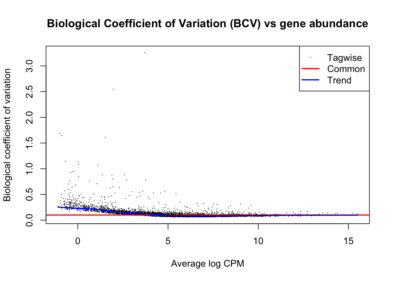
In general, the trend in the NB dispersions should decrease smoothly with increasing abundance. This is because the expression of high-abundance genes is expected to be more stable than that of low-abundance genes. Any substantial increase at high abundances may be indicative of batch effects or trended biases. The value of the trended NB dispersions should range between 0.005 to 0.05 for laboratory-controlled biological systems like mice or cell lines, though larger values will be observed for patient-derived data (> 0.1)
For the QL dispersions, estimation can be performed using the glmQLFit function. This returns a DGEGLM object containing the estimated values of the GLM coefficients for each gene
##         WT.unstressed    WT.EtOH msn24dd.unstressed msn24dd.EtOH
## YIL170W    -15.068482 -13.101209         -15.870351   -13.205823
## YFL056C    -11.085690 -11.011274         -11.067649   -10.422839
## YAR061W    -13.740855 -13.295251         -13.363022   -13.356496
## YGR014W     -8.497729  -8.741701          -8.410553    -8.658257
## YPR031W    -10.545308 -11.887166         -10.448351   -11.862097
## YIL003W    -10.634552 -12.066082         -10.716773   -11.974343
EB squeezing of the raw dispersion estimators towards the trend reduces the uncertainty of the final estimators. The extent of this moderation is determined by the value of the prior df, as estimated from the data. Large estimates for the prior df indicate that the QL dispersions are less variable between genes, meaning that stronger EB moderation can be performed. Small values for the prior df indicate that the dispersions are highly variable, meaning that strong moderation would be inappropriate
Setting robust=TRUE in glmQLFit is strongly recommended. This causes
glmQLFit to estimate a vector of df.prior values, with lower values for
outlier genes and larger values for the main body of genes.
6.10 Testing for differential expression
The final step is to actually test for significant differential expression in each gene, using the QL F-test. The contrast of interest can be specified using the makeContrasts function. Here, genes are detected that are DE between the stressed and unstressed. This is done by defining the null hypothesis as heat stressed - unstressed = 0.
# generate contrasts we are interested in learning about
my.contrasts <- makeContrasts(EtOHvsMOCK.WT = WT.EtOH - WT.unstressed,
                     EtOHvsMOCK.MSN24dd = msn24dd.EtOH - msn24dd.unstressed,
                     EtOH.MSN24ddvsWT = msn24dd.EtOH - WT.EtOH,
                     MOCK.MSN24ddvsWT = msn24dd.unstressed - WT.unstressed,
                     EtOHvsWT.MSN24ddvsWT = (msn24dd.EtOH-msn24dd.unstressed)-(WT.EtOH-WT.unstressed),
                     levels=design)

# This contrast looks at the difference in the stress responses between mutant and WT
res <- glmQLFTest(fit, contrast = my.contrasts[,"EtOHvsWT.MSN24ddvsWT"])## Coefficient: 1*WT.unstressed -1*WT.EtOH -1*msn24dd.unstressed 1*msn24dd.EtOH
## ORF SGD GENENAME logFC logCPM F PValue
## YMR105C YMR105C S000004711 PGM2 -6.840813 9.704453 1607.7248 2.914040e-24
## YMR196W YMR196W S000004809 <NA> -5.153688 8.359888 876.6109 5.583121e-21
## YKL035W YKL035W S000001518 UGP1 -3.840032 10.778897 868.0539 5.645453e-21
## YDR516C YDR516C S000002924 EMI2 -4.006779 9.078562 794.9919 1.647596e-20
## YBR126C YBR126C S000000330 TPS1 -3.455623 9.805436 692.5104 8.800860e-20
## YLR258W YLR258W S000004248 GSY2 -4.863023 8.245400 680.1030 1.095491e-19
## YPR149W YPR149W S000006353 NCE102 -4.239323 7.945052 789.5545 1.161902e-19
## YDR001C YDR001C S000002408 NTH1 -2.889227 7.075130 650.0294 1.893273e-19
## YHL021C YHL021C S000001013 AIM17 -4.206852 6.877514 634.5432 3.509719e-19
## YML100W YML100W S000004566 TSL1 -7.117435 9.813990 1002.5280 5.617293e-19
## FDR
## YMR105C 1.636233e-20
## YMR196W 1.056641e-17
## YKL035W 1.056641e-17
## YDR516C 2.312813e-17
## YBR126C 9.320117e-17
## YLR258W 9.320117e-17
## YPR149W 9.320117e-17
## YDR001C 1.328841e-16
## YHL021C 2.189675e-16
## YML100W 3.154110e-16# generate a beautiful table for the pdf/html file.
topTags(res, n=Inf) |> data.frame() |>
arrange(FDR) |>
mutate(logFC=round(logFC,2)) |>
# mutate(across(where(is.numeric), signif, 3)) |>
mutate_if(is.numeric, signif, 3) |>
remove_rownames() |>
reactable(
searchable = TRUE,
showSortable = TRUE,
columns = list(ORF = colDef(
cell = function(value) {
# Render as a link
url <-
sprintf("https://www.yeastgenome.org/locus/%s", value)
htmltools::tags$a(href = url, target = "_blank", as.character(value))
}
))
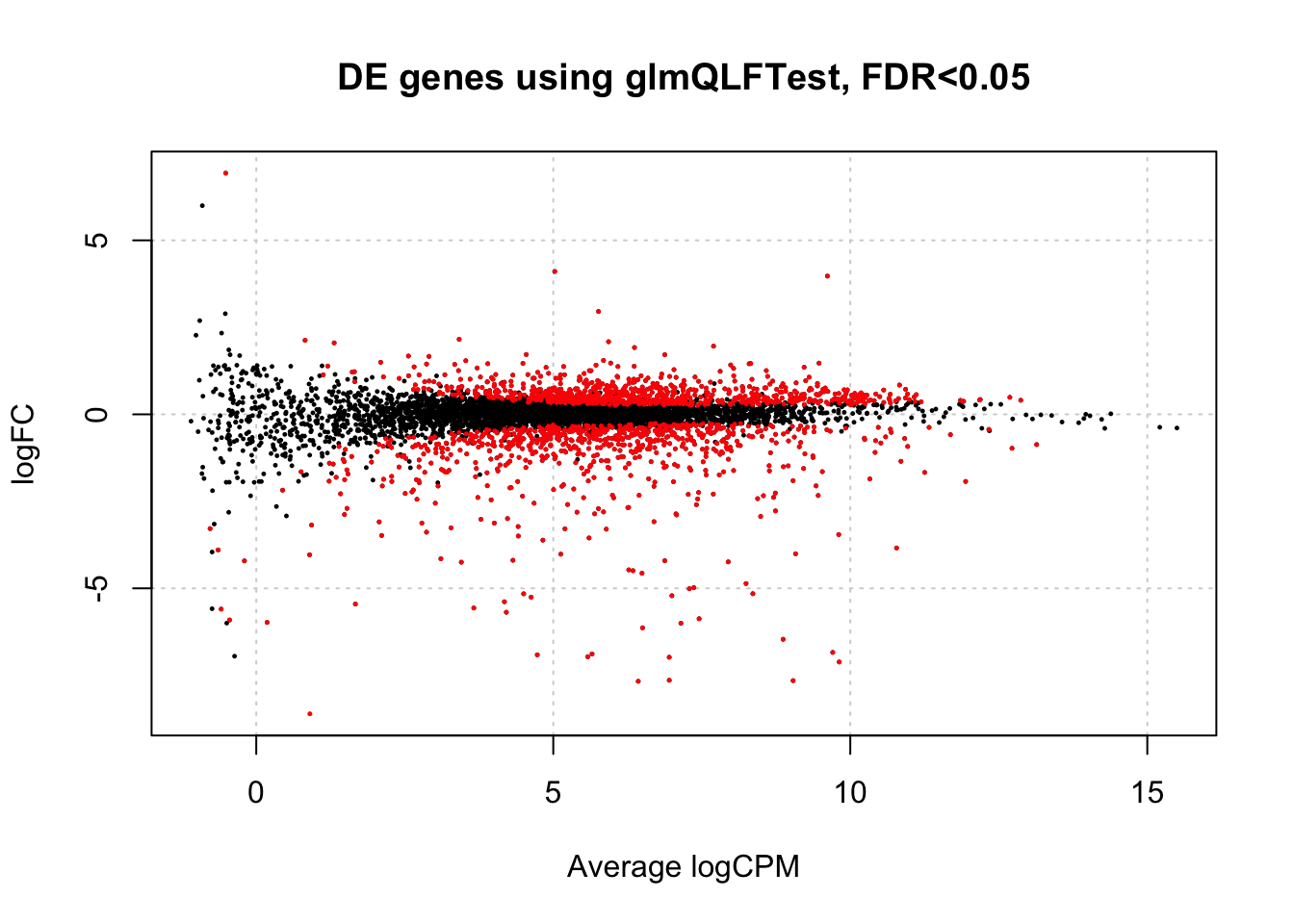
)is.de <- decideTestsDGE(res,
p.value=0.05,
lfc = 0) # this allows you to set a cutoff, BUT...
# if you want to compare against a FC that isn't 0, should use glmTreat instead.
summary(is.de)## 1*WT.unstressed -1*WT.EtOH -1*msn24dd.unstressed 1*msn24dd.EtOH
## Down 761
## NotSig 4031
## Up 823Let’s take a quick look at the differential expression
Here is how we can save our output file(s).
# Choose topTags destination
dir_output_edgeR <-
  path.expand("~/Desktop/Genomic_Data_Analysis/Analysis/edgeR/")
if (!dir.exists(dir_output_edgeR)) {
  dir.create(dir_output_edgeR, recursive = TRUE)
}

# for shairng with others, the topTags output is convenient.
topTags(res, n = Inf) |> data.frame() |>
  arrange(desc(logFC)) |>
  mutate(logFC = round(logFC, 2)) |>
  # mutate(across(where(is.numeric), signif, 3)) |>
  mutate_if(is.numeric, signif, 3) |>
  write_tsv(x=_, file = paste0(dir_output_edgeR, "yeast_topTags_edgeR.tsv"))

# for subsequent analysis, let's save the res object as an R data object.
saveRDS(object = res, file = paste0(dir_output_edgeR, "yeast_res_edgeR.Rds"))

# we might also want our y object list
saveRDS(object = y, file = paste0(dir_output_edgeR, "yeast_y_edgeR.Rds"))
6.11 Looking at all contrasts at once
If we want results from all contrasts, we need to loop through them in edgeR, and them combine the results We will look more at the results of this in a later activity.
# One way is to not specify just one contrast, like this:
res_all <- glmQLFTest(fit, contrast = my.contrasts)

res_all |>
  topTags(n=Inf) |>
  data.frame() |>
  head()
## ORF SGD GENENAME logFC.EtOHvsMOCK.WT
## YDR516C YDR516C S000002924 EMI2 7.037159
## YGR008C YGR008C S000003240 STF2 7.232023
## YNL141W YNL141W S000005085 AAH1 -8.225571
## YLR258W YLR258W S000004248 GSY2 7.555246
## YMR105C YMR105C S000004711 PGM2 7.634455
## YER103W YER103W S000000905 SSA4 7.769421
## logFC.EtOHvsMOCK.MSN24dd logFC.EtOH.MSN24ddvsWT logFC.MOCK.MSN24ddvsWT
## YDR516C 3.030381 -4.7165805 -0.7098017
## YGR008C 2.020311 -6.1176166 -0.9059042
## YNL141W -9.063807 -0.9710603 -0.1328248
## YLR258W 2.692224 -5.2388431 -0.3758203
## YMR105C 0.793642 -6.9808751 -0.1400617
## YER103W 7.122431 -0.7957057 -0.1487160
## logFC.EtOHvsWT.MSN24ddvsWT logCPM F PValue FDR
## YDR516C -4.0067788 9.078562 3135.887 2.130681e-32 6.237991e-29
## YGR008C -5.2117124 6.996589 3125.389 2.221902e-32 6.237991e-29
## YNL141W -0.8382356 7.190029 2964.658 4.298774e-32 8.045873e-29
## YLR258W -4.8630228 8.245400 2746.906 1.115331e-31 1.399179e-28
## YMR105C -6.8408134 9.704453 2722.673 1.245930e-31 1.399179e-28
## YER103W -0.6469897 10.594970 2535.965 3.026744e-31 2.832528e-28# alternatively, we can loop to get DE genes in each contrast.
# here we are just saving which genes are DE per contrast
decideTests_edgeR_tmp <- list()
for (i in 1:ncol(my.contrasts)){
current.res <- glmQLFTest(fit, contrast = my.contrasts[,paste0(dimnames(my.contrasts)$Contrasts[i])])
# current.res <- eBayes(current.res)
decideTests_edgeR_tmp[[i]] <- current.res |> decideTests(p.value = 0.05, lfc = 0) |>
as.data.frame()
}
decideTests_edgeR <- list_cbind(decideTests_edgeR_tmp) |>
rownames_to_column("gene")
head(decideTests_edgeR)## gene -1*WT.unstressed 1*WT.EtOH -1*msn24dd.unstressed 1*msn24dd.EtOH
## 1 YIL170W 1 1
## 2 YFL056C 0 1
## 3 YAR061W 0 0
## 4 YGR014W -1 -1
## 5 YPR031W -1 -1
## 6 YIL003W -1 -1
## -1*WT.EtOH 1*msn24dd.EtOH -1*WT.unstressed 1*msn24dd.unstressed
## 1 0 0
## 2 1 0
## 3 0 0
## 4 0 0
## 5 0 0
## 6 0 0
## 1*WT.unstressed -1*WT.EtOH -1*msn24dd.unstressed 1*msn24dd.EtOH
## 1 0
## 2 1
## 3 0
## 4 0
## 5 0
## 6 0# save this file for future analysis
write_tsv(decideTests_edgeR, "~/Documents/GitHub/GenomicDataAnalysis_Fa23/analysis/yeast_decideTests_allContrasts_edgeR.tsv")
# for subsequent analysis, let's also save the res_all object as an R data object.
saveRDS(object = res_all, file = paste0(dir_output_edgeR, "yeast_res_all_edgeR.Rds"))6.12 Questions
Question 1: How many genes were upregulated and downregulated in the contrast we looked at in todays activity? Be sure to clarify the cutoffs used for determining significance.
Question 2: Which gene has the lowest pvalue with a postive log2 fold change?
Question 3: Choose one of the contrasts in my.contrasts that we didn’t
test together, and identify the top 3 most differentially expressed
genes.
Question 4: In the contrast you chose, give a brief description of the biological interpretation of that contrast.
Question 5: In the example above, we tested for differential expression of any magnitude. Often, we only care about changes of at least a certain magnitude. In this case, we need to use a different command. using the same data, test for genes with differential expression of at least 1 log2 fold change using the glmTreat function in edgeR. How do these results compare to DE genes without a logFC cutoff?
6.13 A template set of code chunks for doing this is below:
We already loaded in the salmon counts as the object counts
above. This code chunk just re-downloads that same file.
path_salmon_counts <- 'https://github.com/clstacy/GenomicDataAnalysis_Fa23/raw/main/data/ethanol_stress/counts/salmon.gene_counts.merged.nonsubsamp.tsv'

counts <- read.delim(
    path_salmon_counts,
    sep = "\t",
    header = T,
    row.names = 1
  )
# We are reusing the sample_metadata, group, etc that we assigned above
# create DGEList with salmon counts
y <- DGEList(counts, group=group)
colnames(y) <- sample_metadata$Sample
# add gene names
y$genes <- AnnotationDbi::select(org.Sc.sgd.db,keys=rownames(y),
columns="GENENAME")## 'select()' returned 1:1 mapping between keys and columns# filter low counts
keep <- rowSums(cpm(y) > 60) >= 4
y <- y[keep,]
# calculate norm factors
y <- calcNormFactors(y)
# estimate dispersion
y <- estimateDisp(y, design, robust=TRUE)
# generate the fit
fit <- glmQLFit(y, design, robust=TRUE)
# Note that, unlike other edgeR functions such as glmLRT and glmQLFTest,
# glmTreat can only accept a single contrast.
# If contrast is a matrix with multiple columns, then only the first column will be used.
# Implement a test against FC at least 1 the test our contrast of interest
tr <- glmTreat(fit,
contrast = my.contrasts[,"EtOHvsWT.MSN24ddvsWT"],
lfc=1)
# generate a beautiful table for the pdf/html file.
topTags(tr, n = Inf) |>
data.frame() |>
arrange(FDR) |>
mutate(logFC = round(logFC, 2)) |>
# mutate(across(where(is.numeric), signif, 3)) |>
mutate_if(is.numeric, signif, 3) |>
remove_rownames() |>
reactable(
searchable = TRUE,
showSortable = TRUE,
columns = list(ORF = colDef(
cell = function(value) {
# Render as a link
url <-
sprintf("https://www.yeastgenome.org/locus/%s", value)
htmltools::tags$a(href = url, target = "_blank", as.character(value))
}
))
)# write the table to a tsv file
topTags(tr, n=Inf) |>
data.frame() |>
arrange(FDR) |>
mutate(logFC=round(logFC,2)) |>
# mutate(across(where(is.numeric), signif, 3)) |>
mutate_if(is.numeric, signif, 3) |>
write_tsv(x=_, file = paste0(dir_output_edgeR, "yeast_lfc1topTags_edgeR.tsv"))
# summarize the DE genes
is.de_tr <- decideTestsDGE(tr, p.value=0.05)
summary(is.de_tr)## 1*WT.unstressed -1*WT.EtOH -1*msn24dd.unstressed 1*msn24dd.EtOH
## Down 106
## NotSig 2255
## Up 11# visualize results
plotSmear(tr, de.tags=rownames(tr)[is.de_tr!=0])
title(main="DE genes using glmTreat with logFC cutoff")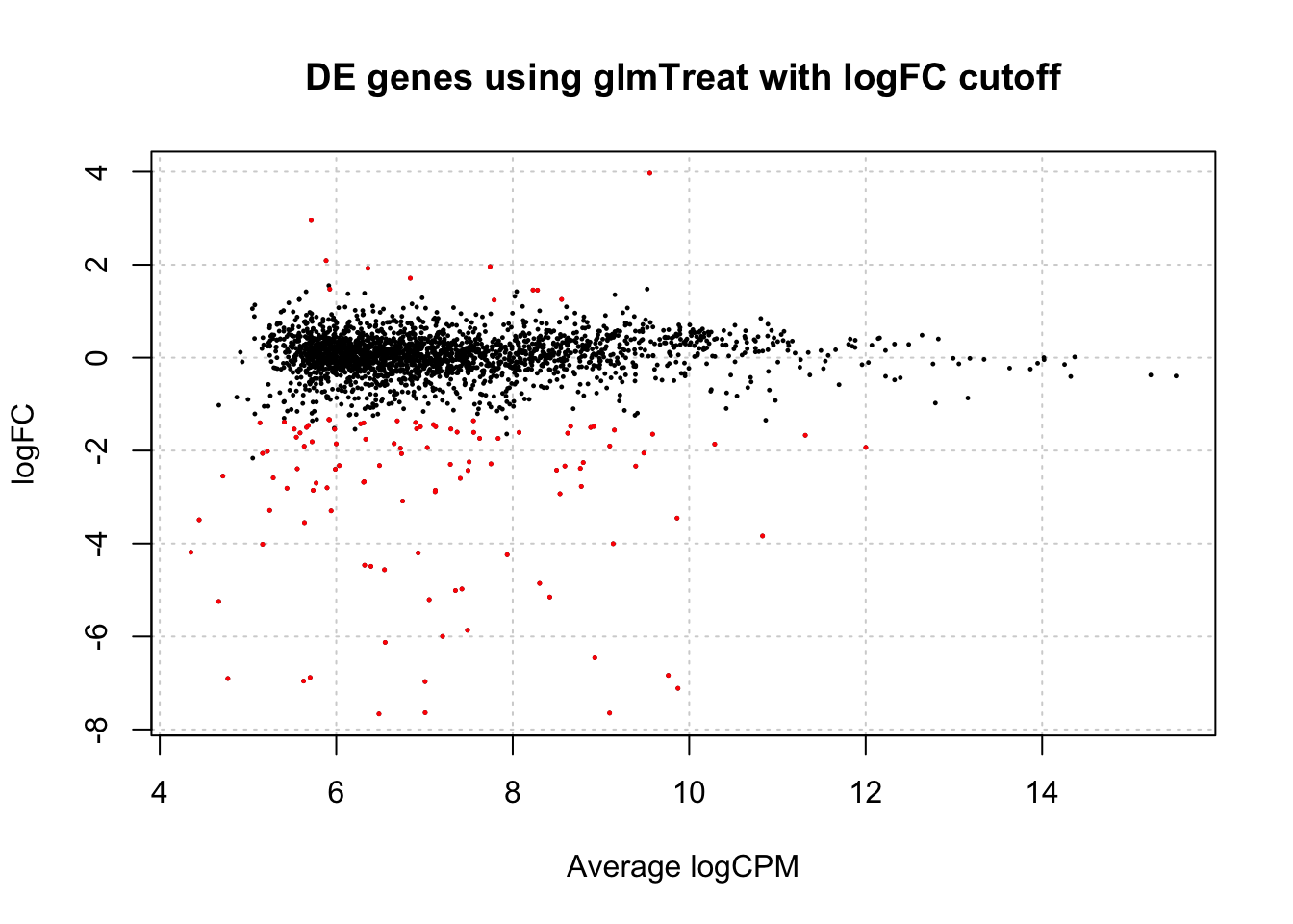
Be sure to knit this file into a pdf or html file once you’re finished.
System information for reproducibility:
R version 4.3.1 (2023-06-16)
Platform: aarch64-apple-darwin20 (64-bit)
locale: en_US.UTF-8||en_US.UTF-8||en_US.UTF-8||C||en_US.UTF-8||en_US.UTF-8
attached base packages: stats4, stats, graphics, grDevices, utils, datasets, methods and base
other attached packages: edgeR(v.3.42.4), limma(v.3.56.2), reactable(v.0.4.4), webshot2(v.0.1.1), statmod(v.1.5.0), Rsubread(v.2.14.2), ShortRead(v.1.58.0), GenomicAlignments(v.1.36.0), SummarizedExperiment(v.1.30.2), MatrixGenerics(v.1.12.3), matrixStats(v.1.0.0), Rsamtools(v.2.16.0), GenomicRanges(v.1.52.1), Biostrings(v.2.68.1), GenomeInfoDb(v.1.36.4), XVector(v.0.40.0), BiocParallel(v.1.34.2), Rfastp(v.1.10.0), org.Sc.sgd.db(v.3.17.0), AnnotationDbi(v.1.62.2), IRanges(v.2.34.1), S4Vectors(v.0.38.2), Biobase(v.2.60.0), BiocGenerics(v.0.46.0), clusterProfiler(v.4.8.2), ggVennDiagram(v.1.2.3), tidytree(v.0.4.5), igraph(v.1.5.1), janitor(v.2.2.0), BiocManager(v.1.30.22), pander(v.0.6.5), knitr(v.1.44), here(v.1.0.1), lubridate(v.1.9.3), forcats(v.1.0.0), stringr(v.1.5.0), dplyr(v.1.1.3), purrr(v.1.0.2), readr(v.2.1.4), tidyr(v.1.3.0), tibble(v.3.2.1), ggplot2(v.3.4.4), tidyverse(v.2.0.0) and pacman(v.0.5.1)
loaded via a namespace (and not attached): splines(v.4.3.1), later(v.1.3.1), bitops(v.1.0-7), ggplotify(v.0.1.2), polyclip(v.1.10-6), lifecycle(v.1.0.3), rprojroot(v.2.0.3), vroom(v.1.6.4), processx(v.3.8.2), lattice(v.0.21-9), MASS(v.7.3-60), crosstalk(v.1.2.0), magrittr(v.2.0.3), sass(v.0.4.7), rmarkdown(v.2.25), jquerylib(v.0.1.4), yaml(v.2.3.7), cowplot(v.1.1.1), chromote(v.0.1.2), DBI(v.1.1.3), RColorBrewer(v.1.1-3), abind(v.1.4-5), zlibbioc(v.1.46.0), ggraph(v.2.1.0), RCurl(v.1.98-1.12), yulab.utils(v.0.1.0), tweenr(v.2.0.2), GenomeInfoDbData(v.1.2.10), enrichplot(v.1.20.0), ggrepel(v.0.9.4), codetools(v.0.2-19), DelayedArray(v.0.26.7), DOSE(v.3.26.1), ggforce(v.0.4.1), tidyselect(v.1.2.0), aplot(v.0.2.2), farver(v.2.1.1), viridis(v.0.6.4), jsonlite(v.1.8.7), ellipsis(v.0.3.2), tidygraph(v.1.2.3), tools(v.4.3.1), treeio(v.1.24.3), Rcpp(v.1.0.11), glue(v.1.6.2), gridExtra(v.2.3), xfun(v.0.40), qvalue(v.2.32.0), websocket(v.1.4.1), withr(v.2.5.1), fastmap(v.1.1.1), latticeExtra(v.0.6-30), fansi(v.1.0.5), digest(v.0.6.33), timechange(v.0.2.0), R6(v.2.5.1), gridGraphics(v.0.5-1), colorspace(v.2.1-0), GO.db(v.3.17.0), jpeg(v.0.1-10), RSQLite(v.2.3.1), utf8(v.1.2.3), generics(v.0.1.3), data.table(v.1.14.8), graphlayouts(v.1.0.1), httr(v.1.4.7), htmlwidgets(v.1.6.2), S4Arrays(v.1.0.6), scatterpie(v.0.2.1), pkgconfig(v.2.0.3), gtable(v.0.3.4), blob(v.1.2.4), hwriter(v.1.3.2.1), shadowtext(v.0.1.2), htmltools(v.0.5.6.1), bookdown(v.0.36), fgsea(v.1.26.0), scales(v.1.2.1), png(v.0.1-8), snakecase(v.0.11.1), ggfun(v.0.1.3), rstudioapi(v.0.15.0), tzdb(v.0.4.0), reshape2(v.1.4.4), rjson(v.0.2.21), nlme(v.3.1-163), cachem(v.1.0.8), RVenn(v.1.1.0), parallel(v.4.3.1), HDO.db(v.0.99.1), pillar(v.1.9.0), grid(v.4.3.1), vctrs(v.0.6.4), promises(v.1.2.1), archive(v.1.1.5), evaluate(v.0.22), cli(v.3.6.1), locfit(v.1.5-9.8), compiler(v.4.3.1), rlang(v.1.1.1), crayon(v.1.5.2), reactR(v.0.5.0), interp(v.1.1-4), ps(v.1.7.5), plyr(v.1.8.9), fs(v.1.6.3), stringi(v.1.7.12), viridisLite(v.0.4.2), deldir(v.1.0-9), munsell(v.0.5.0), lazyeval(v.0.2.2), GOSemSim(v.2.26.1), Matrix(v.1.6-1.1), hms(v.1.1.3), patchwork(v.1.1.3), bit64(v.4.0.5), KEGGREST(v.1.40.1), memoise(v.2.0.1), bslib(v.0.5.1), ggtree(v.3.8.2), fastmatch(v.1.1-4), bit(v.4.0.5), downloader(v.0.4), ape(v.5.7-1) and gson(v.0.1.0)